<?xml version="1.0" encoding="utf-8"?><feed xmlns="http://www.w3.org/2005/Atom" ><generator uri="https://jekyllrb.com/" version="4.3.4">Jekyll</generator><link href="https://duane321.github.io/feed.xml" rel="self" type="application/atom+xml" /><link href="https://duane321.github.io/" rel="alternate" type="text/html" /><updated>2026-09-22T17:49:14+00:00</updated><id>https://duane321.github.io/feed.xml</id><title type="html">DJ Rich</title><subtitle>Personal website of DJ Rich. Articles on machine learning, statistics, and financial engineering.</subtitle><author><name>Duane Rich</name></author><entry><title type="html">AI Inference Platforms: A Practical Guide</title><link href="https://duane321.github.io/concepts/ai-tool-reviews/ai-inference/" rel="alternate" type="text/html" title="AI Inference Platforms: A Practical Guide" /><published>2025-05-18T00:00:00+00:00</published><updated>2025-05-18T00:00:00+00:00</updated><id>https://duane321.github.io/concepts/ai-tool-reviews/ai-inference</id><content type="html" xml:base="https://duane321.github.io/concepts/ai-tool-reviews/ai-inference/"><![CDATA[<p class="center"><img src="https://duane321.github.io/assets/images/posts/ai_inference/inference_layer.png" alt="Inference Layer" style="width: 100%" /></p>
<p>In recent years, the focus of AI innovation has shifted from research-heavy model training to optimized inference, where the goal is to retrieve AI model responses quickly, cheaply, and in large volume. 
Optimizing these is essential for profitable AI products that attract users and scale, explaining the industry’s new emphasis.</p>

<p>In this article, we will unpack the AI inference landscape, emphasizing two types of critical service platforms beyond proprietary model providers: <strong>Managed AI Inference APIs</strong> and <strong>DIY (Do It Yourself) GPU Infrastructure</strong>. We will explore their cost, performance, and operational implications to inform how enterprises choose between them. To do this, we will provide an approximate framework for understanding this inference landscape and discuss how companies have progressed through it.</p>

<h2 id="why-ai-inference-matters">Why AI Inference Matters</h2>

<p>Despite what news coverage may lead you to believe, the most common challenge of AI builders emerges post-training in deploying models to users. <em>Inference</em> describes the process where trained models produce predictions or responses, often in real-time. Increasingly, users expect AI products to be cheap, reliable, responsive, and high volume, which translates into extreme standards for the AI inference layer.</p>

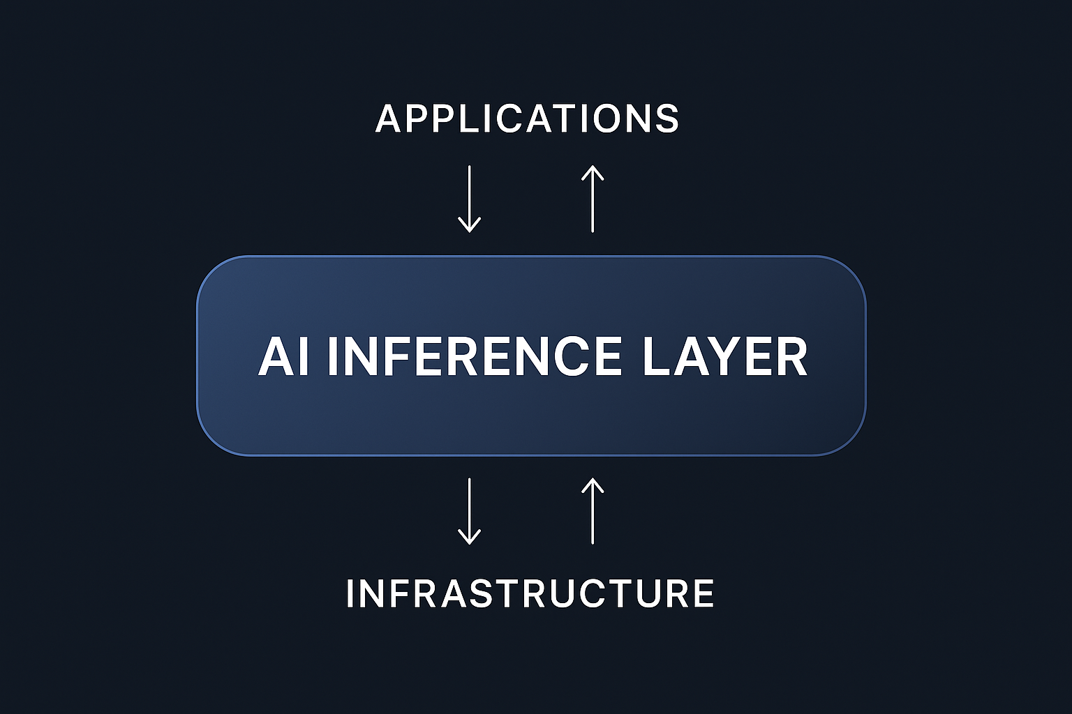
<p>To be exact, the <em>AI inference layer</em> refers to the full stack of services, hardware, and software that sit between a trained model on disk and the end-user request for a prediction. More generally, it refers to all companies and products which participate in this layer.</p>

<p>The complexity of scaling AI inference stems from two intersecting forces. First, companies must weigh trade offs across the stack—balancing flexibility, control, and simplicity—just as they do when choosing between frontend frameworks or database systems. Different workloads and engineering needs demand different levels of abstraction. Second, organizations move through an AI maturity curve. Early-stage teams prioritize speed and ease of use, often relying on proprietary APIs. As they scale and cost pressures grow, they shift<sup id="fnref:1"><a href="#fn:1" class="footnote" rel="footnote" role="doc-noteref">1</a></sup> toward managed APIs for open-source models. Eventually, more advanced teams should transition to DIY GPU Infrastructure to maximize performance and control. These vertical and horizontal forces combine to shape how companies adopt and evolve their inference platforms.</p>

<h2 id="three-categories-of-inference-services">Three Categories of Inference Services</h2>

<p>We find the following chart to be a useful, approximate view of the AI inference landscape:</p>

<p class="center"><img src="https://duane321.github.io/assets/images/posts/ai_inference/chart_1.png" alt="Platform Types" style="width: 100%" />
<span class="figure-caption">Platform types and their broad features</span></p>

<h2 id="proprietary-apis-powerful-polished-and-pricey">Proprietary APIs: Powerful, Polished, and Pricey</h2>

<p>Proprietary APIs from hyperscalers and foundation model creators—like OpenAI (ChatGPT), Anthropic (Claude), and Google DeepMind (Gemini)—offer direct access to their own frontier models through cloud-hosted endpoints. We see the following as their key advantages of the alternatives:</p>

<blockquote>
  <p><strong>Key Benefits</strong>:</p>

  <ul>
    <li>
      <p><strong>Model Quality</strong>: Access to the most advanced models on the market, often with early access to new releases.</p>
    </li>
    <li>
      <p><strong>Zero Infrastructure Lift</strong>: Fully hosted APIs abstract away all deployment, orchestration, and scaling concerns.</p>
    </li>
    <li>
      <p><strong>Enterprise-Grade Ecosystem</strong>: Deep integration with cloud platforms, plus support for security, compliance, and SLAs.</p>
    </li>
    <li>
      <p><strong>Developer Experience</strong>: Rich SDKs, detailed documentation, and support designed for fast integration.</p>
    </li>
  </ul>
</blockquote>

<p>Despite the ease of use, these platforms come with constraints. Pricing is significantly higher due to embedded IP costs. Model weights are inaccessible, fine-tuning is limited, and vendor lock-in can become a concern as usage grows and dependencies deepen.</p>

<blockquote>
  <p><strong>Ideal Users</strong>: Proprietary APIs are ideal for well funded startups, innovation labs, or corporate teams launching early AI experiments. For example, if you’re building a beta version of a customer service chatbot and need best-in-class performance without hiring an ML team, OpenAI or Anthropic is the fastest path to market. Think: “one PM, one frontend dev, one API key”.</p>
</blockquote>

<h2 id="managed-ai-inference-apis-efficient-cost-effective-and-flexible">Managed AI Inference APIs: Efficient, Cost-Effective, and Flexible</h2>

<p>Managed AI inference APIs, provided by platforms like Together.ai, Fireworks.ai, and Replicate, offer a balanced solution between ease of use and cost efficiency. These platforms host open-source and fine-tuned models—such as LLaMA, Mistral, and Mixtral—via performant, developer-friendly APIs.</p>

<blockquote>
  <p><strong>Key Benefits</strong>:</p>

  <ul>
    <li>
      <p><strong>Cost Efficiency</strong>: Lower prices per token by avoiding proprietary model licensing.</p>
    </li>
    <li>
      <p><strong>Flexibility</strong>: Support for model selection, parameter tuning, and user-provided fine-tunes.</p>
    </li>
    <li>
      <p><strong>Performance Optimization</strong>: Techniques like batching and speculative decoding improve latency and throughput.</p>
    </li>
    <li>
      <p><strong>Ease of Use</strong>: APIs simplify scaling and deployment without requiring users to manage infrastructure.</p>
    </li>
  </ul>
</blockquote>

<p>Together.ai and Fireworks.ai, for instance, prioritize rapid inference speeds, high uptime, and a broad catalog of supported models, catering to developers who value performance and variety. Others, like Replicate, focus on ease of use, while platforms such as Anyscale offer scalability for enterprise workloads</p>

<blockquote>
  <p><strong>Ideal Users</strong>: Managed APIs are great for startups or scale-ups that have validated product-market fit and need to scale cost-effectively. For instance, if you’re running a SaaS platform with embedded AI features—like an edtech tool that summarizes reading material—and you’re hitting $50K/month in OpenAI bills, switching to Fireworks or Together with LLaMA models may cut your cost by 10x with minimal migration work.</p>
</blockquote>

<h2 id="diy-gpu-infrastructure-maximum-control-deep-cost-savings">DIY GPU Infrastructure: Maximum Control, Deep Cost Savings</h2>

<p>DIY GPU Infrastructure providers—including RunPod, Lambda Labs, Vast.ai, and Modal—offer raw or semi-managed GPU access for teams that want complete control over model deployment. Users configure everything from runtime environments to model hosting using their preferred tools and frameworks.</p>

<blockquote>
  <p><strong>Key Benefits</strong>:</p>

  <ul>
    <li>
      <p><strong>Lowest Compute Costs</strong>: Access to bare-metal GPUs at rates well below hyperscaler pricing.</p>
    </li>
    <li>
      <p><strong>Full Customization</strong>: Control over every layer—from model weights to system architecture.</p>
    </li>
    <li>
      <p><strong>Scalability</strong>: Ideal for high-volume inference, fine-tuning, or complex deployment pipelines.</p>
    </li>
    <li>
      <p><strong>Vendor Flexibility</strong>: Many providers support spot instances, shared GPUs, and user-owned containers.</p>
    </li>
  </ul>
</blockquote>

<p>This category demands strong technical expertise. Users are responsible for uptime, orchestration, and operational tuning. While some providers ease setup with prebuilt containers or notebooks, success requires considerable ML engineering experience.</p>

<blockquote>
  <p><strong>Ideal Users</strong>: DIY GPU Infrastructure is best for technical AI-native teams with strong infra capabilities and tight cost control needs. For example, if you’re operating a workflow automation agent, demand is growing fast, and you have ML engineers on staff, switching to RunPod or Lambda is probably the right choice. It could lower batch inference cost by ~80%, and it permits fine-tuning, for sharping your model to the specific task. For this category, think: “we built our own orchestration layer, and our infra team cares about cents per token.”</p>
</blockquote>

<h2 id="how-to-choose-inference-platforms">How to Choose Inference Platforms</h2>

<p>Choosing an AI inference platform also depends strongly on where the company is in its AI product development. That is, it is a function of AI operational maturity, how far the product has moved from experimental to scaled deployment. This is a well traveled path, albeit at very different speeds. From this perspective, we see the AI inference categories as:</p>

<blockquote>
  <ol>
    <li>
      <p><strong>Proprietary APIs</strong> are great for fast prototyping. You get access to the best models with zero infrastructure lift.</p>
    </li>
    <li>
      <p><strong>Managed Inference APIs</strong> are the next step when costs start to rise. You keep the simplicity of APIs but gain more control and lower token costs by switching to open-source models.</p>
    </li>
    <li>
      <p><strong>DIY GPU Infrastructure</strong> is the final stop for experienced teams that need the lowest costs, the most control, and/or strict privacy guarantees.</p>
    </li>
  </ol>
</blockquote>

<p>Next, we will walk through how this might look like in practice.</p>

<h2 id="ai-native-startups-from-idea-to-infrastructure-in-12-months">AI-Native Startups: From Idea to Infrastructure in 12 Months</h2>

<p>Startups typically begin with proprietary APIs like OpenAI or Anthropic. It’s the fastest way to launch—no infrastructure, no orchestration, just plug-and-play endpoints that let small teams ship fast. But growth brings pressure. Within months, many teams run into what we call <em>inference shock</em>—costs scale with usage, and $100K+ monthly API bills aren’t uncommon.</p>

<p>At that point, it’s wise to migrate to Managed Inference APIs like Together or Fireworks. These platforms offer up to 10x savings by serving open-source models with optimized infrastructure. Teams still use simple APIs, but gain more control over model choice, decoding parameters, and batching behavior.</p>

<p>Eventually, some teams outgrow even managed APIs. If you’re running a high-scale LLM product—or need fine-tuned privacy, latency, or cost control—your next move is DIY GPU Infrastructure. It’s the lowest-cost, highest-control option, but requires serious MLOps.</p>

<h2 id="enterprises-same-path-slower-pace">Enterprises: Same Path, Slower Pace</h2>

<p>Traditional companies follow the same pattern—but over longer timelines.</p>

<p>They start with proprietary APIs to test ideas safely. These platforms require no infra lift and carry little legal or operational risk—perfect for proofs of concept like internal chatbots or summarization tools.</p>

<p>As pilots mature, cost and compliance come into play. Enterprises shift to Managed APIs that offer better economics and more flexibility, often in private cloud or VPC setups.</p>

<p>Finally, for production-critical workloads, especially in healthcare, finance, or regulated environments, some move to DIY GPU Infrastructure. Whether on-prem or in isolated cloud environments, this gives teams maximal control over cost, performance, and data residency.</p>

<h2 id="a-modeling-exercise-what-does-20-million-tokens-cost">A Modeling Exercise: What Does 20 Million Tokens Cost?</h2>

<blockquote>
  <p>To ground this discussion, we modeled a representative workload: 20 million tokens of inference.</p>
</blockquote>

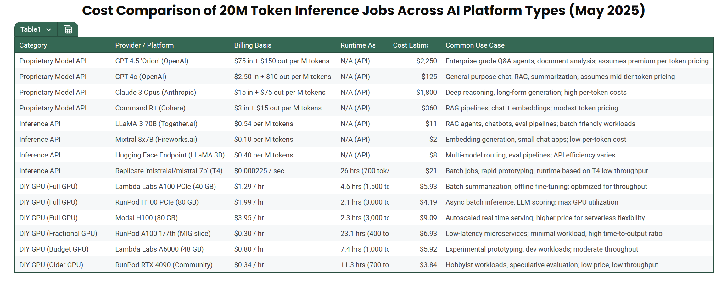
<p>That’s equivalent to 10,000 user queries with 2,000-token responses each, enough to power a summarization tool or a RAG product. This scale is common for startups transitioning out of experimentation or for larger teams running realistic pre-production tests. The point of this benchmark isn’t to name the cheapest provider. Instead, it shows how cost depends on four core variables: platform type, model architecture, latency needs, and optimization strategy.</p>

<p>The table below offers a directional snapshot (as of May 2025) across several providers. These aren’t exact quotes, but they reflect real-world pricing ranges and architectural patterns.</p>

<p class="center"><img src="https://duane321.github.io/assets/images/posts/ai_inference/cost_comparison.png" alt="Platform Types" style="width: 100%" />
<span class="figure-caption">Cost Comparison of 20M Token Inference</span></p>

<h2 id="why-api-token-prices-vary">Why API Token Prices Vary</h2>

<p>While API costs are simple to calculate, the actual price per token varies heavily depending on business model, infrastructure, and workload pattern:</p>

<blockquote>
  <ul>
    <li>
      <p><strong>Model Type &amp; IP</strong>: Proprietary models like GPT-4.5 or Claude 3 Opus come with high IP markups to cover R&amp;D costs. Open-source models like LLaMA 3 or Mixtral, by contrast, are far cheaper to serve.</p>
    </li>
    <li>
      <p><strong>Batching &amp; Throughput</strong>: Providers optimize behind the scenes. For batch jobs (e.g., document summarization), token costs are low due to efficient GPU utilization. For real-time apps (e.g., chatbots), compute is underused between requests, raising costs per token.</p>
    </li>
    <li>
      <p><strong>Platform Overhead</strong>: Proprietary APIs bundle extras like SLAs, customer support, and compliance guarantees. These drive up margins. Managed APIs like Together or Fireworks keep overhead lower but may offer fewer enterprise-grade features.</p>
    </li>
    <li>
      <p><strong>Latency Sensitivity</strong>: Low-latency requirements (e.g., streaming output or tight response times) reduce batching opportunities and increase GPU hold time, leading to higher per-token costs.</p>
    </li>
    <li>
      <p><strong>Autoscaling &amp; Monitoring</strong>: Some platforms include observability, routing, and autoscaling in the price; others charge for it separately or bake it into higher base rates.</p>
    </li>
  </ul>
</blockquote>

<p>In other words: the price is heavily shaped by technical, operational, and business factors behind the scenes.</p>

<blockquote>
  <p>The best approach is to measure it empirically. If it’s a batch job, 20M tokens might take just a few minutes. If it’s real-time at 60 tokens/sec, it’s a totally different story.</p>
</blockquote>

<p>With that in mind, the runtime and cost estimates in the next section should be viewed as directional benchmarks, not absolute truths. They’re built on throughput and GPU utilization assumptions (e.g. 1–2M tokens/hour for large LLMs), and aim to help compare relative cost profiles across providers, not predict your exact bill.</p>

<p>In production? Always benchmark on your actual stack.</p>

<h2 id="cost-formulas-for-ai-inference">Cost Formulas for AI Inference</h2>

<p>To give a sense of how these costs are determined in practice, we can break down the two main pricing approaches: DIY GPU rental and API token pricing.</p>

<h3 id="diy-gpu-platform-hour-based">DIY GPU Platform (hour-based)</h3>

<p>The economics of DIY GPU Infrastructure is a straightforward function of resource time and efficiency:</p>

\[\textrm{Cost} = \textrm{GPU Hourly Rate} \times \frac{\textrm{Total Tokens}}{\textrm{Throughput}\times\textrm{GPU Utilization} \times 3600}\]

<p>where:</p>
<ul>
  <li><strong>GPU Hourly Rate</strong> = hourly price of the rented GPU (e.g., $1.99/hr for RunPod H100)</li>
  <li><strong>Throughput</strong> = average number of tokens processed per second (heavily model and batch size dependent).</li>
  <li><strong>GPU Utilization</strong> = the fraction of time a GPU is actively executing instructions.</li>
</ul>

<p>This simple formula highlights how optimization strategies like batching, speculative decoding, and quantization can directly reduce the cost of GPU-based inference.</p>

<h3 id="managed-api-platform-token-based">Managed API Platform (token-based)</h3>

<p>At first glance, API pricing appears more predictable:</p>

\[\textrm{Cost} = \textrm{Total Tokens} \times \textrm{Price Per Token}\]

<p>However, in reality, Price Per Token is not a static number; it is composed of several moving parts. It can be thought of as:</p>

\[\begin{align}
\textrm{Price Per Token} &amp;= \textrm{Base Cost} + \textrm{Infrastructure Cost} \\
&amp;\phantom{=} + \textrm{IP Markup} + \textrm{Batch/Latency Penalty}
\end{align}\]

<p>where:</p>

<ul>
  <li>
    <p><strong>Base Model Cost</strong> reflects the compute cost for serving that model (lowest for open-source models like LLaMA-3, higher for frontier models like GPT-4o).</p>
  </li>
  <li>
    <p><strong>R&amp;D / IP Markup</strong> is added by proprietary model providers to recover R&amp;D investment.</p>
  </li>
  <li>
    <p><strong>Platform Overhead</strong> accounts for features like autoscaling, orchestration, fine-tuning pipelines, and SLAs.</p>
  </li>
  <li>
    <p><strong>Latency / Batch Penalty</strong> represents the inefficiency of serving small requests or latency-sensitive applications where batching can’t be maximized.</p>
  </li>
</ul>

<p>Importantly, these extra layers reflect strategic choices by providers:</p>

<blockquote>
  <p>Enterprise customers may accept premium rates in exchange for reliability, compliance, and customer support.</p>

  <p>Startups or researchers may optimize batch size and latency tolerance to minimize per-token spend.</p>
</blockquote>

<h2 id="conclusion">Conclusion</h2>

<p>Choosing the right AI inference platform is no longer just a technical consideration—it’s a fundamental decision that defines the unit economics and operational scalability of AI-driven businesses. The decision hinges on aligning platform choices with your organization’s current stage of AI maturity, performance requirements, budget constraints, and compliance needs. Real-world inference economics depend critically on optimization strategies, workload characteristics, latency constraints, and model selection—factors best assessed through direct empirical testing. As companies advance along their AI journey, continuously evaluating infrastructure choices and being prepared to transition between platform types will help ensure sustainable growth and long-term competitive advantage in today’s evolving AI landscape.</p>

<hr />
<h3 id="footnotes">Footnotes</h3>

<div class="footnotes" role="doc-endnotes">
  <ol>
    <li id="fn:1">
      <p>or <em>should</em> shift. Hardware and software lock-in frequently prevent companies from transitioning to a more appropriate inference product. <a href="#fnref:1" class="reversefootnote" role="doc-backlink">&#8617;</a></p>
    </li>
  </ol>
</div>]]></content><author><name>Howe Wang</name></author><category term="ai-tool-reviews" /><category term="Post Formats" /><summary type="html"><![CDATA[We breakdown the AI Inference landscape, which is the industry's new optimization focus.]]></summary><media:thumbnail xmlns:media="http://search.yahoo.com/mrss/" url="https://duane321.github.io/assets/images/posts/ai_inference/inference_layer.png" /><media:content medium="image" url="https://duane321.github.io/assets/images/posts/ai_inference/inference_layer.png" xmlns:media="http://search.yahoo.com/mrss/" /></entry><entry><title type="html">Nebius User Experience: A Field Report</title><link href="https://duane321.github.io/concepts/ai-tool-reviews/nebius/" rel="alternate" type="text/html" title="Nebius User Experience: A Field Report" /><published>2025-05-03T00:00:00+00:00</published><updated>2025-05-03T00:00:00+00:00</updated><id>https://duane321.github.io/concepts/ai-tool-reviews/nebius</id><content type="html" xml:base="https://duane321.github.io/concepts/ai-tool-reviews/nebius/"><![CDATA[<p class="center"><img src="https://duane321.github.io/assets/images/posts/nebius/nebius.png" alt="Nebius Office" style="width: 100%" />
<span class="figure-caption">Nebius Office.</span></p>

<p>In the rapidly evolving landscape of enterprise AI and machine learning, specialized cloud platforms are emerging as viable alternatives to traditional hyperscalers like AWS, Azure, and Google Cloud. Nebius—launched in late 2023 by the Nebius Group (formerly part of Yandex)—positions itself as a purpose-built infrastructure provider for AI and generative AI workloads. Real-world feedback highlights both its strengths and growing pains: users praise the self-serve setup, GPU reliability, comprehensive AI stack and flexible pricing, while also pointing to support delays and limited documentation for advanced use cases. For many teams, Nebius fits into a multi-provider strategy, chosen for its cost-performance trade-offs and integration flexibility. This review offers an impartial look at Nebius’s developer experience, compares it with platforms like <a href="/concepts/ai-tool-reviews/coreweave/">CoreWeave</a> and AWS, and evaluates its suitability across different team profiles and AI infrastructure needs.</p>

<h2 id="what-makes-nebius-stand-out">What Makes Nebius Stand Out</h2>

<p>Nebius carves out its niche with a feature set tailored to AI/ML practitioners:</p>

<ul>
  <li>
    <p><strong>Access to Advanced GPUs with NVIDIA Preferred Status</strong>: Nebius provides access to NVIDIA’s most recent GPUs, such as the H100, H200, and the upcoming GB200 NVL72. Nebius benefits from a close relationship with NVIDIA, ensuring early access to advanced accelerators like the Blackwell Ultra platform and enabling optimized AI infrastructure for training and inference.</p>
  </li>
  <li>
    <p><strong>AI Studio and Managed Kubernetes for Simplified Workflows</strong>: Nebius provides AI Studio, a developer-friendly platform that allows teams to deploy their own models or run inference using pre-trained models like Llama 3 and Mistral. With cost-efficient per-token pricing and batch processing support, AI Studio makes it easy to experiment, fine-tune, and scale inference workloads. Complementing this, Nebius’s managed Kubernetes service handles container orchestration, autohealing, and topology-aware scheduling—reducing the operational overhead of scaling and managing infrastructure for AI applications.</p>
  </li>
  <li>
    <p><strong>Pricing Flexibility and Cost Efficiency</strong>: Nebius offers GPU reservations starting at just $2/hour for training, with lower trial rates and per-token pricing for inference. This pricing model delivers estimated savings of 30%+ compared to the hyperscalers. Users can also reserve GPUs in advance to access additional discounts, making it a highly cost-effective option for AI and ML workloads.</p>
  </li>
  <li>
    <p><strong>Comprehensive AI Stack</strong>: Nebius offers an end-to-end AI platform purpose-built for large-scale ML workloads, developed by an engineering team that previously built Yandex’s internal AI infrastructure. Key components include managed MLflow for experiment tracking, a custom Kubernetes operator for Slurm (Soperator) enabling autoscaling and GPU job orchestration, and AI Studio for fine-tuning and inference on models like Llama 3 and Mistral with per-token pricing and batch support.</p>
  </li>
  <li>
    <p><strong>Data Sensitivity Support with EU Location Benefits</strong>: Nebius ensures secure GPU access for enterprises with strict data policies by operating within encrypted virtual private networks (VPNs), meaning sensitive data—like personal information or trade secrets—stays on-premises without needing to migrate to a public cloud; its EU-based data centers in Finland and Paris further enhance compliance with stringent regulations like GDPR, simplify data residency requirements, and offer low-latency performance for regional teams, all while maintaining top-tier privacy standards.</p>
  </li>
</ul>

<h2 id="what-to-watch-for">What to Watch For</h2>

<ul>
  <li>
    <p><strong>Narrower Ecosystem for General Cloud Workloads</strong>: Nebius is purpose-built for AI and machine learning tasks, but its ecosystem lacks the breadth of services found in more mature platforms like AWS or Databricks. While it provides a managed ClickHouse service for analytics, broader offerings such as fully managed databases, business intelligence tools, or integrated ETL pipelines are limited. This often requires teams to supplement with external tools for non-AI workloads, reducing workflow cohesion.</p>
  </li>
  <li>
    <p><strong>Support and Reliability</strong>: While Nebius offers core support services, some users have reported slower response times compared to major providers like AWS or CoreWeave. This can introduce friction for teams running time-sensitive or production-critical workloads, especially during peak demand or infrastructure issues.</p>
  </li>
  <li>
    <p><strong>Inference Optimization Gap</strong>: Nebius trails Run:ai, a leader in advanced inference optimization, as it lacks Run:ai’s dynamic GPU allocation, model compression, and intelligent orchestration, which ensure minimal latency and high throughput for latency-critical tasks like autonomous driving; despite Nebius AI Studio’s competitive speed and cost-efficiency (up to 50% lower than competitors), its optimization capabilities are less robust for time-sensitive workloads.</p>
  </li>
  <li>
    <p><strong>Scalability and Maturity Risks</strong>: With a current GPU footprint of around 20,000 (targeting 35,000–60,000), Nebius is rapidly scaling but remains a newer entrant. This raises valid concerns about its ability to handle peak demand and maintain long-term platform stability.</p>
  </li>
</ul>

<h2 id="who-should-use-nebius">Who Should Use Nebius?</h2>

<p>Nebius aligns well with specific team needs:</p>

<ul>
  <li>
    <p><strong>Compute-Intensive Startups and Scale-ups</strong>: Ideal for teams building generative AI applications, training large models, or running high-throughput inference workloads. Nebius offers top-tier NVIDIA GPUs (H100, H200) with InfiniBand connectivity, and caters especially well to startups and scale-ups operating with $2M–$3M budgets by providing flexible pricing, low-cost reservations, and access to cloud credit programs like the AI Discovery Award (up to $100K).</p>
  </li>
  <li>
    <p><strong>Teams Seeking Streamlined AI Tools</strong>: Nebius’s AI Studio and managed Kubernetes services simplify workflows, allowing innovation-driven groups to focus on model development and deployment without extensive infrastructure management.</p>
  </li>
  <li>
    <p><strong>Global Teams</strong>: With data centers in Finland, Paris, Kansas City Missouri, and upcoming facilities in New Jersey and Iceland, Nebius ensures low-latency access and supports compliance with regional data regulations, benefiting distributed teams operating across different geographies.</p>
  </li>
  <li>
    <p><strong>Enterprises with Sensitive Data</strong>: Nebius offers features like VPN support to secure GPU access, aligning with stringent data policies and providing enterprises with the necessary tools to maintain data integrity and confidentiality.</p>
  </li>
</ul>

<h2 id="who-might-find-nebius-challenging-to-use">Who Might Find Nebius Challenging to Use?</h2>

<ul>
  <li>
    <p><strong>Teams Requiring Broader Cloud Services</strong>: Nebius’s focus on AI means limited support for general-purpose infrastructure like managed databases, BI tools, or serverless analytics—often requiring external platforms to fill the gap.</p>
  </li>
  <li>
    <p><strong>Support-Dependent Teams</strong>: Users have noted slower response times compared to hyperscalers or CoreWeave, which can be problematic for time-sensitive workflows.</p>
  </li>
  <li>
    <p><strong>Smaller Teams Without DevOps Expertise</strong>: While powerful, Nebius relies on tools like Kubernetes and Slurm that assume a baseline of operational knowledge, which may be a barrier for lean or non-specialist teams.</p>
  </li>
  <li>
    <p><strong>Risk-Averse Organizations</strong>: As a newer entrant with a smaller global footprint, Nebius may not meet the risk tolerance of enterprises that prioritize long-established providers with extensive compliance and uptime records.</p>
  </li>
</ul>

<h2 id="comparison-to-coreweave-and-hyperscalers">Comparison to CoreWeave and Hyperscalers</h2>

<p>Nebius occupies a unique middle ground between CoreWeave’s compute-focused infrastructure and the full-stack ecosystems of hyperscalers like AWS and Google Cloud. It surpasses CoreWeave in ecosystem development by offering integrated tools such as AI Studio and managed Kubernetes, which simplify model development and deployment. However, it still falls short of the seamless, end-to-end platforms offered by hyperscalers—such as SageMaker, which tightly integrates coding, training, and deployment workflows.</p>

<p>Where Nebius stands out is in pricing flexibility: it offers GPU reservations, predictable per-token inference pricing, and trial discounts that significantly undercut hyperscaler pricing. Through its Explorer Tier, Nebius provides access to high-performance GPUs starting at $1.50 per hour for up to 1,000 GPU hours monthly. Longer-term reservations reduce rates even further—H100s start at $2.00/hour and H200s at $2.30/hour with a three-month commitment—making it an attractive option for cost-conscious AI teams. Overall, Nebius’s pricing is up to 30% lower than hyperscalers, with additional discounts of up to 35% for sustained usage. The discount structure is particularly well-suited to workloads where teams can estimate training requirements in advance. If the size of the training data and the type of model are known upfront, teams can estimate total GPU hours required and reserve capacity accordingly to secure lower pricing. This level of cost predictability makes Nebius an efficient choice for training scenarios with clearly defined compute needs.</p>]]></content><author><name>Howe Wang</name></author><category term="ai-tool-reviews" /><category term="Post Formats" /><summary type="html"><![CDATA[We explore Nebius and the factors to consider when choosing it over the alternatives.]]></summary><media:thumbnail xmlns:media="http://search.yahoo.com/mrss/" url="https://duane321.github.io/assets/images/posts/nebius/nebius_logo.png" /><media:content medium="image" url="https://duane321.github.io/assets/images/posts/nebius/nebius_logo.png" xmlns:media="http://search.yahoo.com/mrss/" /></entry><entry><title type="html">CoreWeave User Experience: A Field Report</title><link href="https://duane321.github.io/concepts/ai-tool-reviews/coreweave/" rel="alternate" type="text/html" title="CoreWeave User Experience: A Field Report" /><published>2025-03-27T00:00:00+00:00</published><updated>2025-03-27T00:00:00+00:00</updated><id>https://duane321.github.io/concepts/ai-tool-reviews/coreweave</id><content type="html" xml:base="https://duane321.github.io/concepts/ai-tool-reviews/coreweave/"><![CDATA[<p>In the fast-evolving world of enterprise AI and machine learning, the demand for specialized cloud solutions is surging. Yet traditional hyper-scalers like AWS, Azure, and Google Cloud often fall short of meeting the needs of specialized AI/ML projects. If you’re an enterprise AI/ML leader, you’ve likely experienced moments when your current provider fails—whether due to lagging performance, rising costs, delayed access to the latest hardware, or a lack of tooling—prompting a search for alternatives. Vendor lock-in can make these challenges even harder. Once your workloads are tightly coupled with a provider’s ecosystem, switching becomes costly and operationally complex, reducing your ability to respond to innovation, improve efficiency, or leverage better infrastructure options elsewhere.</p>

<p>While there’s no shortage of detailed comparisons analyzing provider specs, strategies, and financials, the real challenge remains:</p>

<blockquote>
  <p>As an AI/ML practitioner, how do you actually decide on the right GPU cloud provider?</p>
</blockquote>

<p>We explore the key decision triggers and offer a practical framework to help you make this decision. From our experience and surveying the space, it’s clear that in some cases, a different vendor is the better choice. We’ll kick off with an in-depth look at CoreWeave—a GPU cloud provider known for raw compute, now expanding into developer experience and higher-level tooling. This analysis reflects the current experience and assessments from an enterprise AI/ML team as of March 2025.</p>

<h2 id="what-makes-coreweave-stand-out">What Makes CoreWeave Stand Out</h2>

<p>CoreWeave’s pricing structure is one of its most compelling advantages—particularly when compared to traditional hyper-scalers like AWS. Like many emerging GPU cloud providers, CoreWeave operates in a more dynamic, marketplace-style pricing environment that allows for greater flexibility and negotiation.</p>

<blockquote>
  <p>This often results in 30–50% lower costs for GPU-heavy workloads.</p>
</blockquote>

<p>We go into more detail in the pricing section below, but the takeaway is simple: if you’re training models at scale or running high-throughput inference, providers like CoreWeave can offer meaningful savings over hyperscaler alternatives.</p>

<p>Another key advantage is its immediate access to the latest NVIDIA GPUs—such as the GB200 and H100—typically within weeks of release, a speed that often outpaces competitors. One reason technical leaders pick hyper-scalers is because they assume they have the best capacity. But since hyper-scalers are so well subscribed, this doesn’t mean they offer the best GPU availability. CoreWeave, however, has plenty of scale—32 data centers with over 250,000 GPUs—offering ample room for even massive foundational model training, a critical need for AI/ML leaders facing compute-intensive initiatives.</p>

<p>Performance is another strong point. Unlike hyper-scalers’ virtualized environments, where multiple tenants share resources, CoreWeave uses bare metal servers. This means your code runs directly on dedicated hardware, eliminating virtualization overhead and delivering faster, more predictable performance for GPU-heavy tasks like model training or simulations. Additionally, CoreWeave provides essential managed services—like the CoreWeave Kubernetes Service (CKS) for orchestration and Weights &amp; Biases for experiment tracking—that streamline workflows and support the priorities of AI/ML teams.</p>

<h2 id="what-to-watch-for">What to Watch For</h2>

<p>Despite its strengths, CoreWeave doesn’t offer the full-service ecosystem you’d find with hyper-scalers like AWS, Azure, or Google Cloud.</p>

<blockquote>
  <p>If your project depends on managed databases, integrated analytics, or prebuilt AI platforms like SageMaker or Vertex AI, you’ll need to piece together those components using third-party tools or manage them yourself.</p>
</blockquote>

<p>The onboarding process also creates friction. Rather than a self-service sign-up, you need to schedule a meeting to get started—adding potential delays for teams hoping to spin up infrastructure quickly. And while CoreWeave provides strong building blocks for cloud infrastructure, using them effectively often requires significant technical expertise. Running Kubernetes clusters, managing Slurm-based batch jobs, and optimizing resource allocation all demand familiarity with cloud-native and HPC-style workflows.</p>

<p>Additionally, the absence of prebuilt inference APIs means teams must develop custom solutions or rely on third-party tools that offer pre-deployed inference APIs for popular models, introducing complexity that may hinder smaller teams or those seeking straightforward, streamlined workflows.</p>

<h2 id="who-should-use-coreweave">Who Should Use CoreWeave?</h2>

<p>CoreWeave is ideal for technically proficient teams of ML scientists and DevOps engineers who can effectively utilize its bare metal infrastructure and flexible tools for custom, high-performance workflows. Teams with strong skills in container orchestration (e.g., Kubernetes), workload scheduling (e.g., Slurm), and cluster management will thrive. Its raw computational power is particularly suited for training large models or running complex simulations where control and optimization are prioritized over ease of use. Large-scale projects requiring long-term GPU access will benefit from CoreWeave’s efficiency and volume discounts, especially through multi-year leases. Enterprises or research groups committed to sustained AI/HPC workloads can capitalize on its cost savings and access to advanced hardware.</p>

<h2 id="who-might-find-coreweave-challenging-to-use">Who Might Find CoreWeave Challenging to Use?</h2>

<p>Teams without dedicated infrastructure expertise may find CoreWeave challenging to adopt. Unlike more turnkey platforms, it requires hands-on setup and ongoing management of orchestration and scheduling tools. Small teams, early-stage startups, or non-tech-centric enterprises experimenting with AI may struggle if they lack in-house resources to manage GPU infrastructure. Additionally, CoreWeave’s more rigid onboarding process and focus on compute over end-to-end developer experience means users must take on more operational responsibility. For those seeking a plug-and-play platform or a simplified interface, other providers may offer a more accessible alternative.</p>

<h2 id="a-note-on-pricing">A Note on Pricing</h2>

<p>CoreWeave’s pricing structure stands out as a compelling alternative to hyper-scalers like AWS, offering a blend of flexibility, negotiation room, transparency, and lower overall costs—particularly well-suited for AI/ML workloads.</p>

<blockquote>
  <p>Unlike hyper-scalers, which often break down charges into separate categories like compute, storage, and networking, CoreWeave bills with a per-instance, per-hour pricing model. Each instance bundles GPUs, CPUs, RAM, networking, local NVMe storage, and pre-configured software into a single rate, making costs easier to predict and manage.</p>
</blockquote>

<p>With hyper-scalers, costs can unexpectedly spiral as you scale—between egress fees, premium storage tiers, and unexpected service charges, it becomes difficult to accurately model and forecast spend. For AI/ML teams, especially at startups or non-tech-centric firms, CoreWeave’s flat-rate, bundled approach is a strong differentiator.</p>

<p>As of early 2024, CoreWeave lists an 8x H100 GPU instance at $49.24/hour under its Classic Pricing model. This “sticker price” serves as a baseline in a highly dynamic market where the actual cost varies based on the pricing structure:</p>

<ul>
  <li><strong>Spot Pricing</strong>: The lowest-cost option, offering interruptible rates ideal for non-critical workloads like batch inference. With a one-minute eviction risk, it’s not suitable for training.</li>
  <li><strong>Contract/Reserved Pricing</strong>: Offers guaranteed access with rates locked in from 1 month to 3 years. A middle-ground option balancing reliability and cost, though fewer teams are committing long-term due to rapid market changes.</li>
  <li><strong>On-Demand Pricing</strong>: The most expensive but most flexible option. Ideal for development, testing, or burst workloads when instant access is more important than cost-efficiency.</li>
</ul>

<p>Today’s GPU rental market is in a price war. H100 rates have dropped from $8/hour in 2023 to as low as $1/hour in 2025, according to Cybernews. While these figures don’t reflect CoreWeave-specific pricing, they highlight industry-wide pricing pressure—and why negotiation is critical.</p>

<p>Your key advantage with CoreWeave—and other emerging GPU cloud providers—is the ability to negotiate. Unlike AWS, where discounts are tied to rigid upfront commitments and long-term reserved instances, CoreWeave offers more adaptable contracts and is often quicker to reflect market trends in its pricing. While exact discounts aren’t public, it’s widely recognized that committed customers can negotiate substantial reductions off list prices. A startup may get modest savings, while a large enterprise with multi-year usage can secure deeper cuts.</p>

<p>Estimates vary—some reports suggest CoreWeave can be 30–50% cheaper than hyper-scalers for GPU workloads, and anecdotal claims point to discounts of 50–70% off list rates. The reality likely depends on your specific use case, workload type, and negotiation leverage.</p>

<p>Ultimately, listed prices are just the starting point. Teams that track GPU market benchmarks (e.g. $1–3/hour for H100s) and negotiate flexible, short-term contracts are best positioned to capture cost advantages—especially in a fast-moving market where locking into a multi-year rate today could mean overpaying tomorrow.</p>

<h2 id="our-overview-of-coreweave-tooling">Our Overview of CoreWeave Tooling</h2>

<p>Below is our overview of CoreWeave’s tooling and platform architecture—broken down by segment to highlight what’s included, what stands out technically, and where teams might encounter friction. This breakdown is designed to help enterprise AI/ML teams assess CoreWeave’s strengths and potential challenges across the full stack.</p>

<table>
  <thead>
    <tr>
      <th>Segment</th>
      <th style="text-align: center">What They Offer</th>
      <th style="text-align: center">What They Do Well</th>
      <th style="text-align: center">Technical Origin</th>
      <th style="text-align: center">Challenges</th>
    </tr>
  </thead>
  <tbody>
    <tr>
      <td><strong>Infrastructure</strong></td>
      <td style="text-align: center">Access to GPUs (GB200, H100), 32 data centers, and bare metal servers for high performance. 250,000 GPUs online</td>
      <td style="text-align: center">Delivers great computational power and higher GPU cluster performance than alternative solutions. Model FLOPS Utilization (MFU) exceeding 50% on NVIDIA Hopper GPUs</td>
      <td style="text-align: center">Elite Cloud Services Provider (CSP) within the NVIDIA Partner Network (NPN), ensuring early access to hardware</td>
      <td style="text-align: center">Some users note occasional congestion during peak usage, though it’s rare</td>
    </tr>
    <tr>
      <td><strong>Networking / Interconnect</strong></td>
      <td style="text-align: center">High-performance networking with InfiniBand, BlueField DPUs, and upgraded Ethernet, built for AI and HPC workloads</td>
      <td style="text-align: center">Enables fast, low-latency GPU-to-GPU communication with non-blocking interconnects—ideal for distributed training and inference</td>
      <td style="text-align: center">Built on NVIDIA Quantum-2 InfiniBand, Spectrum switches, and in-house infrastructure</td>
      <td style="text-align: center">N/A</td>
    </tr>
    <tr>
      <td><strong>Container Orchestration</strong></td>
      <td style="text-align: center">CoreWeave Kubernetes Service (CKS), a managed Kubernetes platform optimized for GPU workloads, with out-of-the-box production readiness</td>
      <td style="text-align: center">Simplifies container orchestration with fast spin-up times and strong GPU performance, leveraging familiar Kubernetes tools.</td>
      <td style="text-align: center">Developed initially in-house with Loft Labs using vCluster, integrated directly with CoreWeave’s bare-metal infrastructure for efficiency.</td>
      <td style="text-align: center">May still limit user-facing “ease-of-use” compared to traditional cloud-native Kubernetes services</td>
    </tr>
    <tr>
      <td><strong>Workload Scheduling</strong></td>
      <td style="text-align: center">SUNK for efficient scheduling, Helm chart with GitOps, ideal for HPC/AI training</td>
      <td style="text-align: center">Optimizes resource use, reduces idle compute, seamless batch job management</td>
      <td style="text-align: center">Developed with SchedMD, combines Slurm and Kubernetes, reflects HPC focus</td>
      <td style="text-align: center">Complexity for beginners, potential integration challenge</td>
    </tr>
    <tr>
      <td><strong>AI Development Tools</strong></td>
      <td style="text-align: center">Weights &amp; Biases integration for experiment tracking, model management, collaboration</td>
      <td style="text-align: center">Streamlines ML development, reduces trial-and-error, deep integration, excels in collaborative tracking and visualization</td>
      <td style="text-align: center">Brought through acquisition in March 2025</td>
      <td style="text-align: center">N/A</td>
    </tr>
    <tr>
      <td><strong>Inference Services</strong></td>
      <td style="text-align: center">Serverless inference with autoscaling, raw GPU support for custom setups, and Tensorizer for faster model loading</td>
      <td style="text-align: center">Fast scalable inference with cost-efficient bare-metal GPUs.</td>
      <td style="text-align: center">N/A</td>
      <td style="text-align: center">No prebuilt APIs, custom builds required,</td>
    </tr>
  </tbody>
</table>

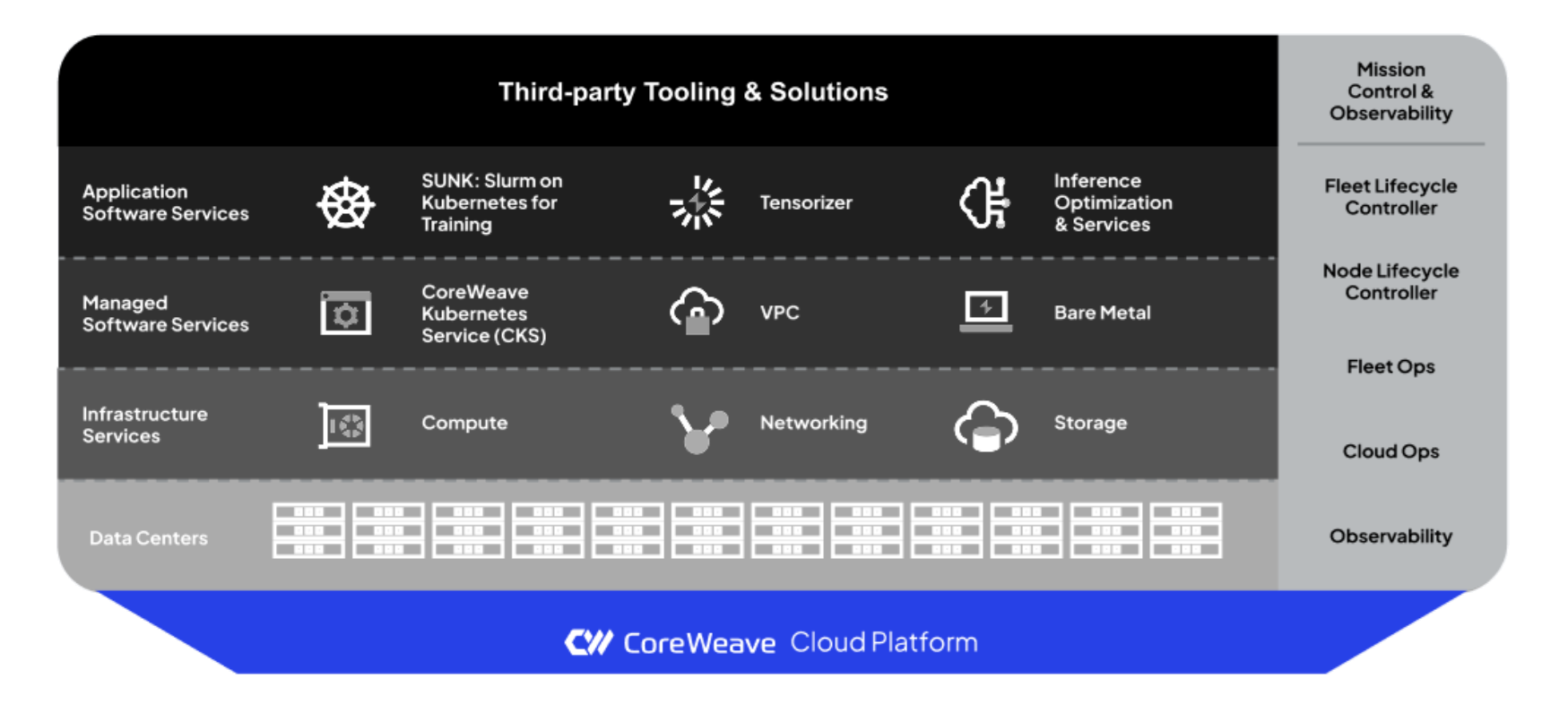
<p>We also find the below graph from CoreWeave to be especially informative about how their product is layered.</p>

<p class="center"><img src="https://duane321.github.io/assets/images/posts/ai_tool_review/coreweave/coreweave_layers.png" alt="CoreWeave Layered Architecture Stack" style="width: 100%" />
<span class="figure-caption">CoreWeave Layered Architecture Stack. <a href="https://www.coreweave.com/blog/coreweave-leads-the-charge-in-ai-infrastructure-efficiency-with-up-to-20-higher-gpu-cluster-performance-than-alternative-solutions">Source</a>.</span></p>]]></content><author><name>Howe Wang</name></author><category term="ai-tool-reviews" /><category term="Post Formats" /><summary type="html"><![CDATA[We explore CoreWeave and the factors to consider when choosing it over AWS, GCP and Azure.]]></summary><media:thumbnail xmlns:media="http://search.yahoo.com/mrss/" url="https://duane321.github.io/assets/images/posts/ai_tool_review/coreweave/coreweave_logo.png" /><media:content medium="image" url="https://duane321.github.io/assets/images/posts/ai_tool_review/coreweave/coreweave_logo.png" xmlns:media="http://search.yahoo.com/mrss/" /></entry><entry><title type="html">BentoML</title><link href="https://duane321.github.io/concepts/ai-tool-reviews/bentoml/" rel="alternate" type="text/html" title="BentoML" /><published>2025-03-12T00:00:00+00:00</published><updated>2025-03-12T00:00:00+00:00</updated><id>https://duane321.github.io/concepts/ai-tool-reviews/bentoml</id><content type="html" xml:base="https://duane321.github.io/concepts/ai-tool-reviews/bentoml/"><![CDATA[<p>In this article, we’ll review BentoML, an open-source platform designed to simplify deploying, managing, and scaling machine learning models. At the end, we’ll provide a one-page PDF summarizing our take.</p>

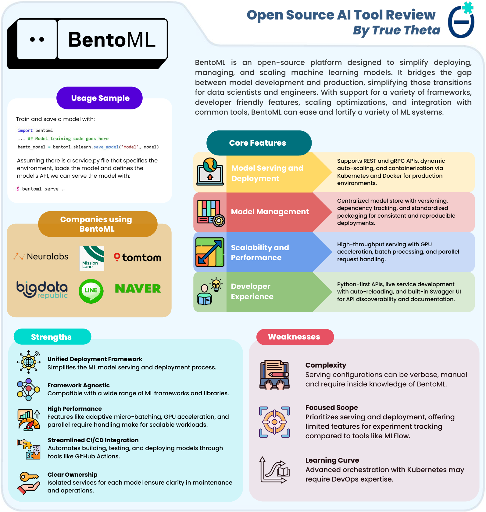
<h2 id="bentoml-serving-and-deployment">BentoML Serving and Deployment</h2>

<p>BentoML addresses a common challenge for data scientists and engineers: the gap between model development and production deployment. It is a persistent source of breakages and frustration. Large companies invest considerable time and money into in-house solutions to minimize this misalignment. BentoML offers an open-source alternative, well tested and adopted by companies. As an example, we find <a href="https://medium.com/mission-lane-tech-blog/mlops-infrastructure-at-mission-lane-7e780d99496e">Mission Lane’s BentoML blog posts</a> to be an illustrative how-to case study.</p>

<p>To do this, BentoML shortens the distance between a data scientist’s model training code and a served model. As a brief illustration, we could have a <code class="language-plaintext highlighter-rouge">save_model.py</code> file that performs:</p>

<div class="language-python highlighter-rouge"><div class="highlight"><pre class="highlight"><code><span class="kn">import</span> <span class="n">bentoml</span>

<span class="p">...</span> <span class="c1">## Model training code goes here
</span><span class="n">bento_model</span> <span class="o">=</span> <span class="n">bentoml</span><span class="p">.</span><span class="n">sklearn</span><span class="p">.</span><span class="nf">save_model</span><span class="p">(</span><span class="sh">'</span><span class="s">model</span><span class="sh">'</span><span class="p">,</span> <span class="n">model</span><span class="p">)</span>
</code></pre></div></div>

<p>Assuming there is a <code class="language-plaintext highlighter-rouge">service.py</code> file that specifies the environment, loads the model, and defines the model’s API, we can run the following in the same directory to serve the model:</p>

<div class="language-bash highlighter-rouge"><div class="highlight"><pre class="highlight"><code><span class="nv">$ </span>bentoml serve <span class="nb">.</span>
</code></pre></div></div>

<p>The model would now be available via an API. BentoML is well tested in this operation, largely eliminating a common source of breakages. For more details, see <a href="https://github.com/bentoml/BentoXGBoost">here</a>.</p>

<h2 id="model-management">Model Management</h2>

<p>BentoML provides a centralized model store with versioning, dependency tracking, and standardized packaging. This makes it easier to catalog models, handle their dependencies, and track their status. This is especially helpful since dependency variations are a common source of production breakages.</p>

<h2 id="scalability-and-performance">Scalability and Performance</h2>

<p>For production models, BentoML offers high-throughput serving with several performance optimizations:</p>

<ul>
  <li><a href="https://docs.bentoml.com/en/latest/get-started/adaptive-batching.html"><strong>Adaptive micro-batching</strong></a> dynamically adjusts batch size and batching intervals based on real-time request patterns. This helps minimize latency during periods of low traffic and increases throughput under higher loads, optimizing resource usage without manual tuning.</li>
  <li><a href="https://docs.bentoml.com/en/latest/build-with-bentoml/gpu-inference.html"><strong>GPU acceleration</strong></a> allows BentoML services to leverage GPUs for faster model inference. BentoML supports assigning specific GPUs or multiple GPUs per service, enabling efficient resource utilization and reduced latency. This is particularly beneficial for compute-intensive models, like LLMs or computer vision models.</li>
  <li><a href="https://docs.bentoml.com/en/latest/build-with-bentoml/parallelize-requests.html"><strong>Parallelized request handling</strong></a> enables BentoML services to process requests concurrently by running multiple worker processes. This improves utilization of multi-core CPUs and GPUs by balancing throughput and resource usage according to workload requirements.</li>
</ul>

<h2 id="developer-experience">Developer Experience</h2>

<p>BentoML prioritizes the developer experience with:</p>
<ul>
  <li>Python-first APIs that feel natural to data scientists.</li>
  <li>Live service development with <a href="https://github.com/bentoml/BentoML/issues/1617#issuecomment-1015984651">auto-reloading</a> for quick iterations.</li>
  <li>A built-in Swagger UI for visualizing, documenting, and interacting with RESTful APIs. This is auto-generated and allows developers to explore API endpoints, test requests, and view responses in the browser.</li>
</ul>

<h2 id="strengths">Strengths</h2>

<p>From our experience and surveying GitHub issues, user feedback, and industry adoption patterns, we believe BentoML’s primary strengths are:</p>

<ul>
  <li><strong>Unified Deployment Framework</strong>: BentoML simplifies the ML model serving and deployment process, providing a consistent workflow, reasonably independent of the underlying ML framework.</li>
  <li><strong>Framework Agnostic</strong>: The platform is compatible with a wide range of ML frameworks and libraries, including scikit-learn, PyTorch, TensorFlow, Hugging Face, and others. This flexibility allows teams to use their preferred tools while maintaining a standardized deployment approach.</li>
  <li><strong>High Performance</strong>: Features like adaptive micro-batching, GPU acceleration, and parallel evaluation allow served models to manage high-volume workloads.</li>
  <li><strong>Streamlined CI/CD Integration</strong>: BentoML integrates well with modern development workflows, allowing for automated building, testing, and deploying of models through tools like GitHub Actions.</li>
  <li><strong>Clear Ownership</strong>: The service-based architecture creates clear boundaries of responsibility, with isolated services for each model ensuring clarity in maintenance and operations.</li>
</ul>

<h2 id="weaknesses">Weaknesses</h2>

<p>We’ve also identified some challenges users should consider:</p>

<ul>
  <li><strong>Complexity</strong>: Writing serving configs can be verbose, manual, and require knowledge of BentoML’s internals. Further, writing custom, non-standard models can require extensive additional code.</li>
  <li><strong>Focused Scope</strong>: BentoML prioritizes serving and deployment, offering limited features for experiment tracking compared to tools like MLflow. Organizations looking for an end-to-end ML platform might need to combine BentoML with other tools for comprehensive coverage of the ML lifecycle, especially for observability.</li>
  <li><strong>Learning Curve</strong>: While BentoML simplifies many aspects of model deployment, advanced orchestration with Kubernetes may still require DevOps expertise. Organizations without this expertise might face implementation challenges.</li>
</ul>

<h2 id="summary">Summary</h2>

<p>To make this discussion portable, we’ve packaged the main points into a downloadable PDF:</p>

<div class="pdf_pc">
	<object data="/assets/images/posts/ai_tool_review/bentoml/bentoml_one_pager.pdf" type="application/pdf" width="100%" height="110%" style="border: none; max-width: 100%; margin-left: auto; margin-right: auto;">
		<iframe src="/assets/images/posts/ai_tool_review/bentoml/bentoml_one_pager.pdf" type="application/pdf" width="100%" height="110%" style="border: none; max-width: 100%; margin-left: auto; margin-right: auto;">
	</iframe>
	<p>
		Your browser does not support PDFs.
		<a href="/assets/images/posts/ai_tool_review/bentoml/bentoml_one_pager.pdf" download="">Download the PDF</a>.
	</p>
	</object>
</div>

<div class="pdf_mobile">
	<div class="mobile_pdf_placeholder">
		<img src="/assets/images/posts/ai_tool_review/bentoml/bentoml_one_pager_pic.png" alt="PDF" />
	</div>
</div>

<p><a href="/assets/images/posts/ai_tool_review/bentoml/bentoml_one_pager.pdf" download="" class="pdf_download_button">Download PDF</a></p>]]></content><author><name>Howe Wang</name></author><category term="ai-tool-reviews" /><category term="Post Formats" /><summary type="html"><![CDATA[A one-page review of BentoML, a platform for deploying and scaling machine learning models.]]></summary><media:thumbnail xmlns:media="http://search.yahoo.com/mrss/" url="https://duane321.github.io/assets/images/posts/ai_tool_review/bentoml/bentoml_logo.png" /><media:content medium="image" url="https://duane321.github.io/assets/images/posts/ai_tool_review/bentoml/bentoml_logo.png" xmlns:media="http://search.yahoo.com/mrss/" /></entry><entry><title type="html">TrueSkill Part 2: Who is the GOAT?</title><link href="https://duane321.github.io/concepts/machine-learning-and-other-topics/true-skill-part-2/" rel="alternate" type="text/html" title="TrueSkill Part 2: Who is the GOAT?" /><published>2025-02-26T00:00:00+00:00</published><updated>2025-02-26T00:00:00+00:00</updated><id>https://duane321.github.io/concepts/machine-learning-and-other-topics/true-skill-part-2</id><content type="html" xml:base="https://duane321.github.io/concepts/machine-learning-and-other-topics/true-skill-part-2/"><![CDATA[<p>In the <a href="/concepts/machine-learning-and-other-topics/true-skill-part-1/">previous post</a>, we argued that the question of ‘Who is the Greatest Of All Time?’ for any competitive game is answerable with an algorithm. They can account for the facts that skills vary over time and many players never played each other in their prime.</p>

<p>To demonstrate, we reviewed the mechanics of the TrueSkill algorithm, invented by a team from Microsoft Research and in response to the inability of the Elo rating system to be applied to multiplayer, multiteam games.</p>

<p>In this post, we’ll use a variant of this algorithm, ‘TrueSkill Through Time,’ and match data to answer the ‘Who is the GOAT?’ question for Tennis, Boxing, and Warcraft 3.</p>

<h2 id="trueskill-through-time">TrueSkill Through Time</h2>

<p>As mentioned at the end of Part 1, the ‘vanilla’ TrueSkill requires some adjustment to properly answer the GOAT question. First, a player’s skill estimate only depends on <em>past</em> data. This is a fair condition if the skill is to be used for forecasting, but it’s suboptimal for the GOAT question. If a player beats another who later becomes a top-tier player, that player’s skill should be revised upward in retrospect. In other words, defeating Mike Tyson in his first professional bout should create a substantial skill boost to the victor.</p>

<p>Second, vanilla TrueSkill indexes time with matches. It treats two matches separated by three days the same as two matches separated by three years. In reality, skills evolve over time, even when no matches occur.</p>

<p>These issues are addressed by the <a href="https://www.microsoft.com/en-us/research/publication/trueskill-through-time-revisiting-the-history-of-chess/">TrueSkill Through Time</a> algorithm. In this analysis, we use <a href="https://trueskillthroughtime.readthedocs.io/en/latest/">the implementation</a> developed by Gustavo Landfried.</p>

<h2 id="tennis">Tennis</h2>

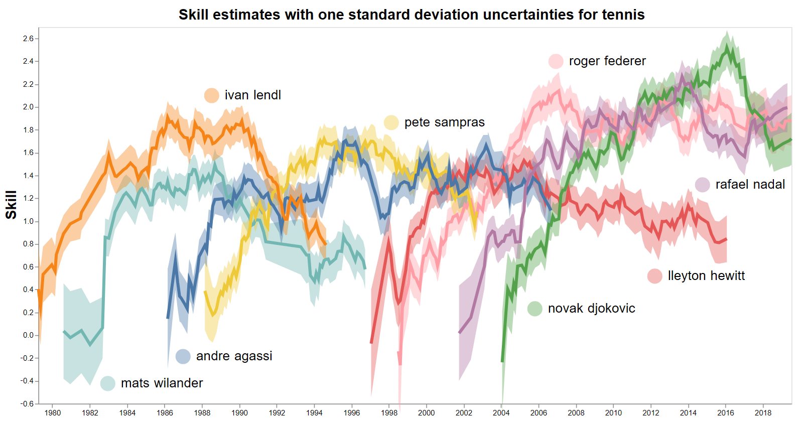
<p>Our first application is to tennis (as <a href="https://trueskillthroughtime.readthedocs.io/en/latest/man/examples.html">Landfried did as well</a>). The code, available <a href="https://github.com/Duane321/true_theta/blob/main/posts/trueskill/tennis.ipynb">here</a>, produces skill estimates over time:</p>

<p class="center"><img src="https://duane321.github.io/assets/images/posts/trueskill/tennis_skills_over_time.png" alt="Tennis Skills" style="width: 100%" />
<span class="figure-caption">Skill estimates, along with one standard deviation uncertainty bands, for some top tennis players over the past four decades.</span></p>

<p>For readability, the skill estimates are shown for select top players over the past forty or so years. Specifically, they come from a dataset of 284,664 matches involving 12,307 players over the past 110 years.</p>

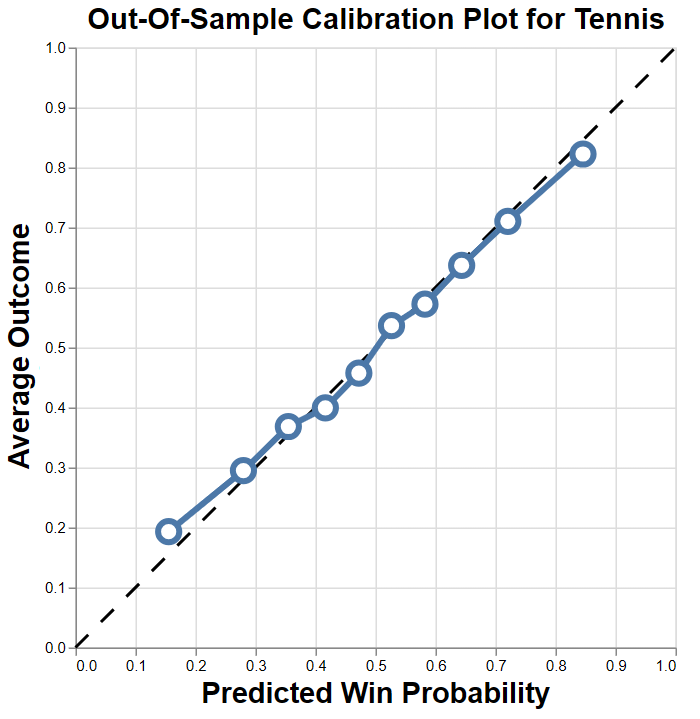
<p>A remaining question is, ‘how do we know these estimates are any good?’ To answer that, we’ve held out the past four years of data and produced the following calibration plot.</p>

<p class="center"><img src="https://duane321.github.io/assets/images/posts/trueskill/tennis_calibration.png" alt="Tennis skill estimate" style="width: 60%" />
<span class="figure-caption">This test-set calibration plot answers the question ‘If the model predicts a win probability of x percent, what is the actual win percentage?’ For a well calibrated model, these numbers should be close; the points plotted should fall along the diagonal line. </span></p>

<p>The model is well calibrated, giving us confidence in its estimates<sup id="fnref:1"><a href="#fn:1" class="footnote" rel="footnote" role="doc-noteref">1</a></sup>. Therefore, we can answer the GOAT question confidently:</p>

<blockquote>
  <p>Established with his 2016 season, <strong>Novak Djokovic</strong> is the greatest of all time. If every player played every other player in their primes, Djokovic is estimated to have the highest win probability.</p>
</blockquote>

<p>As further validation, his 2016 season is <a href="https://en.wikipedia.org/wiki/2016_Novak_Djokovic_tennis_season">noted independently as remarkable</a>.</p>

<h2 id="warcraft-3">Warcraft 3</h2>

<p>Warcraft 3, a classic real time strategy game with a small-but-loyal player base, may seem like an unusual choice relative to tennis and boxing. It was included primarily because it has substantial data. Some players play multiple games a day for many years. Secondarily, I personally have some nostalgia for it and enjoyed the excuse to explore the game’s data.</p>

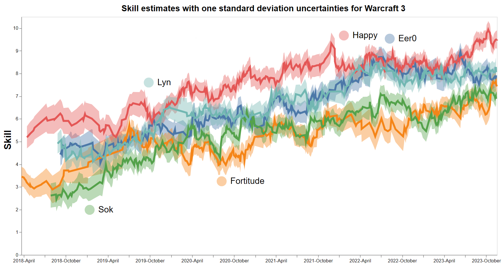
<p>With <a href="https://github.com/Duane321/true_theta/blob/main/posts/trueskill/warcraft3.ipynb">this notebook</a>, we produce the following skill estimates.</p>

<p class="center"><img src="https://duane321.github.io/assets/images/posts/trueskill/warcraft3_skills_over_time.png" alt="Warcraft 3 Skills" style="width: 100%" loading="lazy" />
<span class="figure-caption">Skill estimates of five top players over the past 6 years. </span></p>

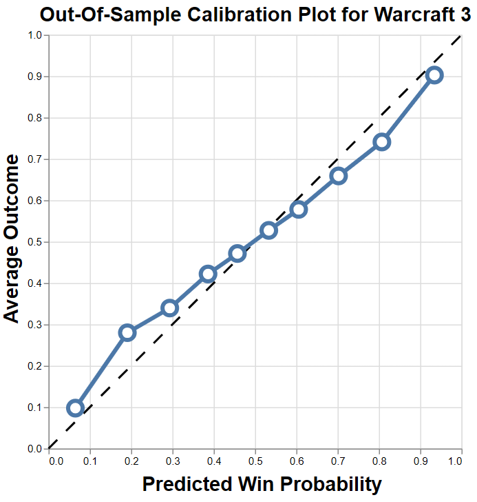
<p>Again, we view the calibration plot to evaluate the model.</p>

<p class="center"><img src="https://duane321.github.io/assets/images/posts/trueskill/warcraft3_calibration.png" alt="Warcraft 3 Calibration Plot" style="width: 60%" loading="lazy" />
<span class="figure-caption">The skill estimates for Warcraft 3 are mostly well calibrated.</span></p>

<p>The model is slightly overconfident with predicted win probabilities between 10-30% or 70-90%. This suggests that the single hyperparameter \(\beta\) may not be flexible enough to capture the game’s noisy dynamics; the level of ‘luck’ may depend on the difference in skills.</p>

<p>Nonetheless, this issue would not change the answer to the GOAT question. We may say confidently:</p>

<blockquote>
  <p>Established in late 2021, <a href="https://liquipedia.net/warcraft/Happy"><strong>Dmitry “Happy” Kostin</strong></a> is the greatest of all time.</p>
</blockquote>

<p>For those experienced with the game, this is not surprising, since Happy has been dominant for nearly a decade.</p>

<h2 id="boxing">Boxing</h2>

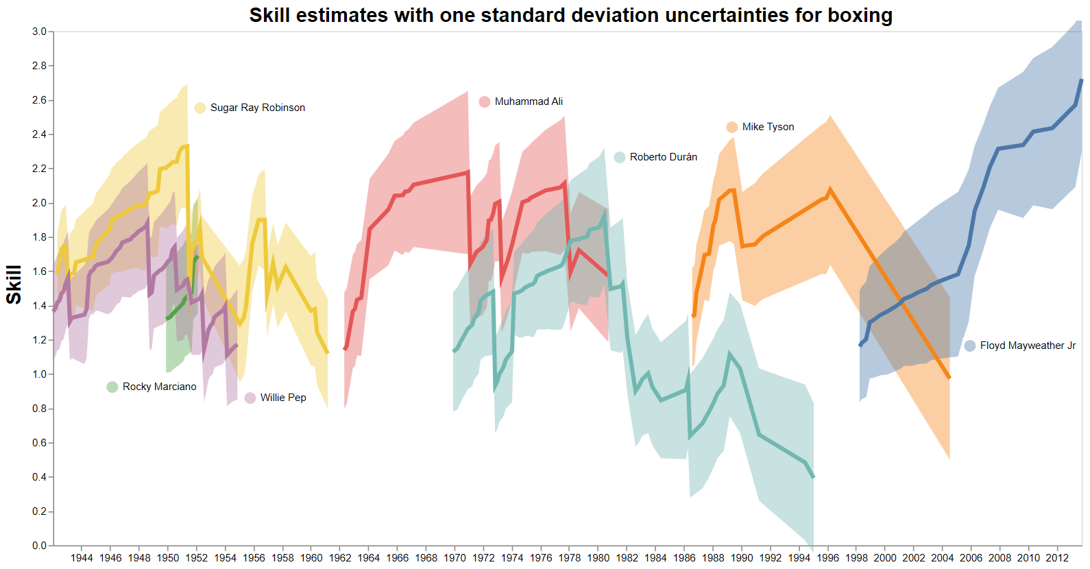
<p>Boxing was the original motivation for the analysis, since ‘Who is the greatest boxer of all time?’ is a fiercely debated question. Rather disappointingly, the data is not as friendly. Using <a href="https://github.com/Duane321/true_theta/blob/main/posts/trueskill/boxing.ipynb">this notebook</a>, we get the following skill estimates.</p>

<p class="center"><img src="https://duane321.github.io/assets/images/posts/trueskill/boxing_skills_over_time.png" alt="Boxing Skills" style="width: 100%" loading="lazy" />
<span class="figure-caption">Skill estimates of some top boxers.</span></p>

<p>The uncertainty bands are significantly wider than in previous cases, and the model linearly interpolates skills over long periods without matches. This follows from the sparsity of the data; boxing matches are much rarer than tennis or Warcraft 3 matches. Over their career, a boxer will have a few dozen fights, whereas some tennis players play thousands of matches.</p>

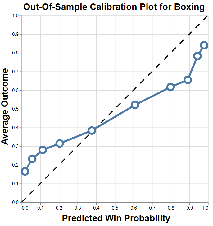
<p>As a result of this sparsity, the model is not especially well calibrated.</p>

<p class="center"><img src="https://duane321.github.io/assets/images/posts/trueskill/boxing_calibration.png" alt="Boxing Calibration Plot" style="width: 60%" />
<span class="figure-caption">The TrueSkill model for boxing is not well calibrated, but there is a strong correlation between predicted and actual win probabilities</span></p>

<p>Despite this, the model seems to rank skill well. According to the calibration plot, an increase in skill corresponds to an increase in test-set win probability. For this, we can have some confidence in the GOAT answer:</p>

<blockquote>
  <p>Due to his undefeated record, including fights with top boxers, <strong>Floyd Mayweather Jr.</strong> is the greatest of all time.</p>
</blockquote>

<p>However, the application to boxing has some notable differences from tennis and Warcraft 3. First, boxing has weight classes, meaning every match is controlled for this variable. Because of this, Floyd Mayweather Jr. in his prime is unlikely to beat heavier boxers in their prime. So ‘greatest of all time’ is really a pound-for-pound greatest, since the data is controlled for weight.</p>

<p>Further, weight classes strongly separate the data. They represent groups within which matches happen frequently, and between which matches are rare. This severely weakens the comparability across weight classes. This is another source of incomparability of boxers from different weight classes.</p>

<h2 id="in-closing">In Closing</h2>

<p>As we’ve seen, the TrueSkill Through Time algorithm—and its variants—really does allow us to tackle one of the most contentious debates in sports: <em>Who is the GOAT?</em> The calibration plots bolster our confidence by showing that the model does predict matches well, and its conclusions align with what seasoned observers of these sports often say. Whether it’s identifying Djokovic’s remarkable peak in tennis, Happy’s dominance in Warcraft 3, or Mayweather’s supremacy in (pound-for-pound) boxing, the results check out. Moreover, other domains, like chess, can be <a href="https://papers.nips.cc/paper_files/paper/2007/file/9f53d83ec0691550f7d2507d57f4f5a2-Paper.pdf">similarly analyzed</a>. After all, wherever structured match data exists, so does the opportunity to learn about the greatest of all time.</p>

<p>Lastly, I’d like to acknowledge the depth of skill estimation. In state-of-the-art applications, much more contextual data can be incorporated than presented here and algorithms can be more finely tuned and evaluated. For those interested in finding the very best algorithm for esports skill estimation in particular, I recommend exploring the <a href="https://github.com/cthorrez/riix">riix</a> package, designed to evaluate and compare algorithms.</p>

<h3 id="references">References</h3>

<ol>
  <li>P. Dangauthier, R. Herbrich, T. Minka, T. Graepel. <a href="https://www.microsoft.com/en-us/research/publication/trueskill-through-time-revisiting-the-history-of-chess/">TrueSkill Through Time: Revisiting the History of Chess</a> In Advances in Neural Information Processing Systems. MIT Press, January 2008.</li>
</ol>

<hr />

<h3 id="footnotes">Footnotes</h3>

<div class="footnotes" role="doc-endnotes">
  <ol>
    <li id="fn:1">
      <p>It should be noted that a good-looking calibration plot is not a complete evaluation of the model. What is missing is the proportions in which the model is giving certain predictions. A perfect model would predict only 0% and 100% and never be wrong. A poor but well calibrated model would predict 50% almost all of the time. In all games, it is unsurprising that the win rate for a random player is 50%. <a href="#fnref:1" class="reversefootnote" role="doc-backlink">&#8617;</a></p>
    </li>
  </ol>
</div>]]></content><author><name>Duane Rich</name></author><category term="machine-learning-and-other-topics" /><category term="Post Formats" /><summary type="html"><![CDATA[We use the TrueSkill algorithm to answer 'Who is the GOAT?' for Boxing, Tennis and Warcraft 3.]]></summary><media:thumbnail xmlns:media="http://search.yahoo.com/mrss/" url="https://duane321.github.io/assets/images/posts/trueskill/tennis_skills_over_time_zoomed.png" /><media:content medium="image" url="https://duane321.github.io/assets/images/posts/trueskill/tennis_skills_over_time_zoomed.png" xmlns:media="http://search.yahoo.com/mrss/" /></entry><entry><title type="html">TrueSkill Part 1: The Algorithm</title><link href="https://duane321.github.io/concepts/machine-learning-and-other-topics/true-skill-part-1/" rel="alternate" type="text/html" title="TrueSkill Part 1: The Algorithm" /><published>2025-02-18T00:00:00+00:00</published><updated>2025-02-19T00:00:00+00:00</updated><id>https://duane321.github.io/concepts/machine-learning-and-other-topics/true-skill-part-1</id><content type="html" xml:base="https://duane321.github.io/concepts/machine-learning-and-other-topics/true-skill-part-1/"><![CDATA[<p>Who is the greatest boxer of all time? Who is the ‘GOAT?’ Is it Muhammad Ali? Mike Tyson? Someone else?</p>

<p>Because they never fought each other, you might say it can’t be known. Indeed, it can’t be <em>known</em>, but it can be estimated.</p>

<p>The absence of a prime Tyson vs prime Ali match does not mean we have no evidence. Something can be inferred from Tyson’s win over Larry Holmes and Larry Holmes’ win over Ali. Additional evidence comes from a chain of two fighters, one who fought Tyson, one who fought Ali and who fought each other. Still more evidence comes from a chain of three fighters, and so on. Collectively, across all chains, there’s substantial evidence to predict the outcome of the Tyson vs Ali fight.</p>

<p>An immediate critique is that Ali fought Holmes at the end of his career and Tyson fought him near his prime. This effect can be handled as well, with an assumption that skill evolves incrementally over time and with experience.</p>

<blockquote>
  <p>Introduced in <a href="https://www.microsoft.com/en-us/research/publication/trueskilltm-a-bayesian-skill-rating-system/" target="_blank" rel="noopener noreferrer">Herbrich et al. (2007)</a>, the <span style="color:#205081"><strong>TrueSkill</strong></span> algorithm captures these effects beautifully. With some extensions, Microsoft deploys it at scale to matchmake many millions of gamers annually. Beyond its applied utility, it is an exceptional victory for Bayesian methods, where simple assumptions and probabilistic reasoning produce accurate estimates of counterfactual matchups.</p>
</blockquote>

<p>Further, the algorithm is game agnostic. All that is needed is when-and-who data on matches. As such, it can be applied to boxing, tennis, chess, MMA, and others. In fact, it can be applied to arbitrarily team multiplayer games, like Halo.</p>

<h2 id="the-elo-rating-system">The Elo Rating System</h2>

<p>To motivate, let’s consider the issue with counting metrics to evaluate skill. If you were to evaluate a chess player’s skill, which metric would you use? Win Rate?</p>

<p>That creates a problem. Win rate doesn’t account for the strength of the opponent. A win rate of 20% against exclusively Magnus Carlsen, arguably the GOAT, is much more impressive than a 90% win rate against an amateur.</p>

<p>This is why the <em>Elo rating system</em> is used for chess and many other two player games.</p>

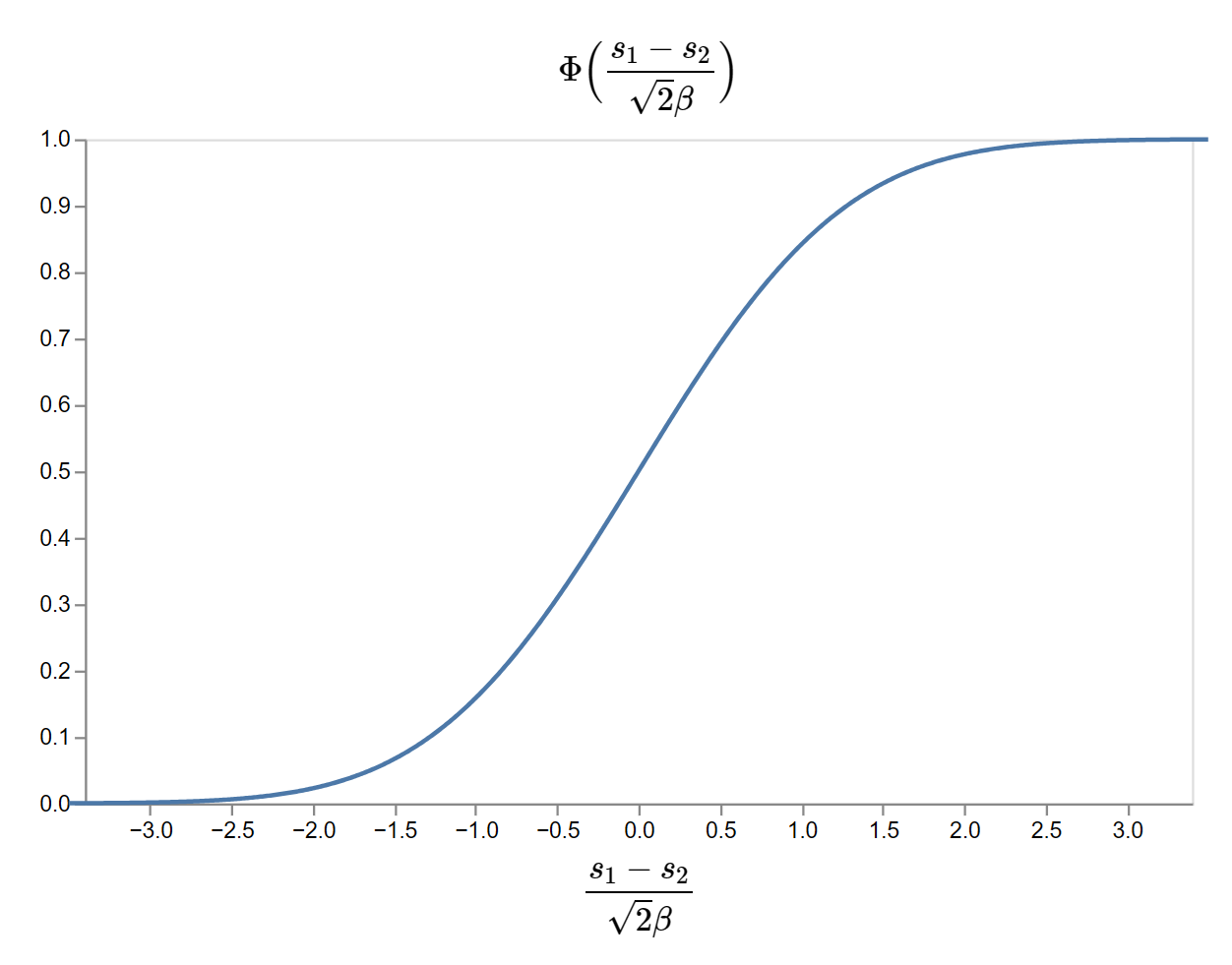
<p>The idea is to assign skill values to players and to model the probability of a win as the difference of their skills. If player 1 has skill \(s_1\) and player 2 has skill \(s_2\), the probability player 1 wins is model as<sup id="fnref:1"><a href="#fn:1" class="footnote" rel="footnote" role="doc-noteref">1</a></sup>:</p>

\[\Phi\Big(\frac{s_1 - s_2}{\sqrt{2}\beta}\Big)\]

<p>where \(\Phi(\cdot)\) is the cumulative density of a standard normal distribution. It looks like:</p>

<p class="center"><img src="https://duane321.github.io/assets/images/posts/trueskill/normal_CDF.png" alt="Normal CDF" style="width: 65%" />
<span class="figure-caption">The cumulative density function of the standard normal distribution. It is chosen for its S-shape, nothing more.</span></p>

<p>The effect is that if player 1 is much more skilled than player 2, \(s_1 - s_2\) is large and positive and the probability of plyer 1 winning is close to one. Similarly, it’s close to zero when player 2 is much more skilled than player 1. \(\beta\) is a tunable parameter to set what counts as ‘large’.</p>

<p>This becomes useful when we have \(N\) players who have played each other many times. Per maximum likelihood estimation, we can estimate \(s_1, s_2, \cdots, s_N\) by applying the win probability to all observed games and finding those that make the observations most likely.</p>

<blockquote>
  <p>The key is that skills are estimated <em>jointly</em>. They are inferred simultaneously, from observed match outcomes to skill differences to skill values. This means all skills are determined in relation to each other, such that skill differences explain the data maximally well.</p>
</blockquote>

<p>Admittedly, I’ve oversimplified things. In practice, skills evolve over time and the optimization can be converted into convenient update rules to be applied after each match. Regardless, this online procedure does not contradict the skills’ relative definition.</p>

<h2 id="problems-with-elo">Problems with Elo</h2>

<p>In 2005, Microsoft Research considered Elo when looking to improve their matchmaking for XBox Live and Halo specifically.</p>

<blockquote>
  <p>Elo wasn’t the answer for a few reasons:</p>

  <ul>
    <li><strong>There is no measure of uncertainty.</strong> Surely, there should be something separating the skill of a player who has played once and another who has played 100+ times.</li>
    <li><strong>It only applies to two player games.</strong> Complicating things, Halo normally involves more than two players.</li>
    <li><strong>There are no teams.</strong> Halo could involve free-for-all matches or team-based play.</li>
  </ul>
</blockquote>

<h2 id="trueskill-what-it-does">TrueSkill: What It Does</h2>

<p>In 2006, TrueSkill was invented in response, and it has since stood the test of time.</p>

<p>To understand it, we’ll begin with TrueSkill’s assumptions. It assumes the data is produced by a certain data generating process or simulation. Rather than describing it precisely and in its full generality, I’ll illustrate the essentials.</p>

<p>Suppose there are \(N\) players playing over \(M\) matches. In fact, <em>with</em> loss of generality, we’re treating the match index like a time index, as though there were one match per timestep, involving all players. Further, each match could be a free-for-all, or with two-player teams, or three-player teams. This is also a loss of generality, since TrueSkill works with arbitrary teams.</p>

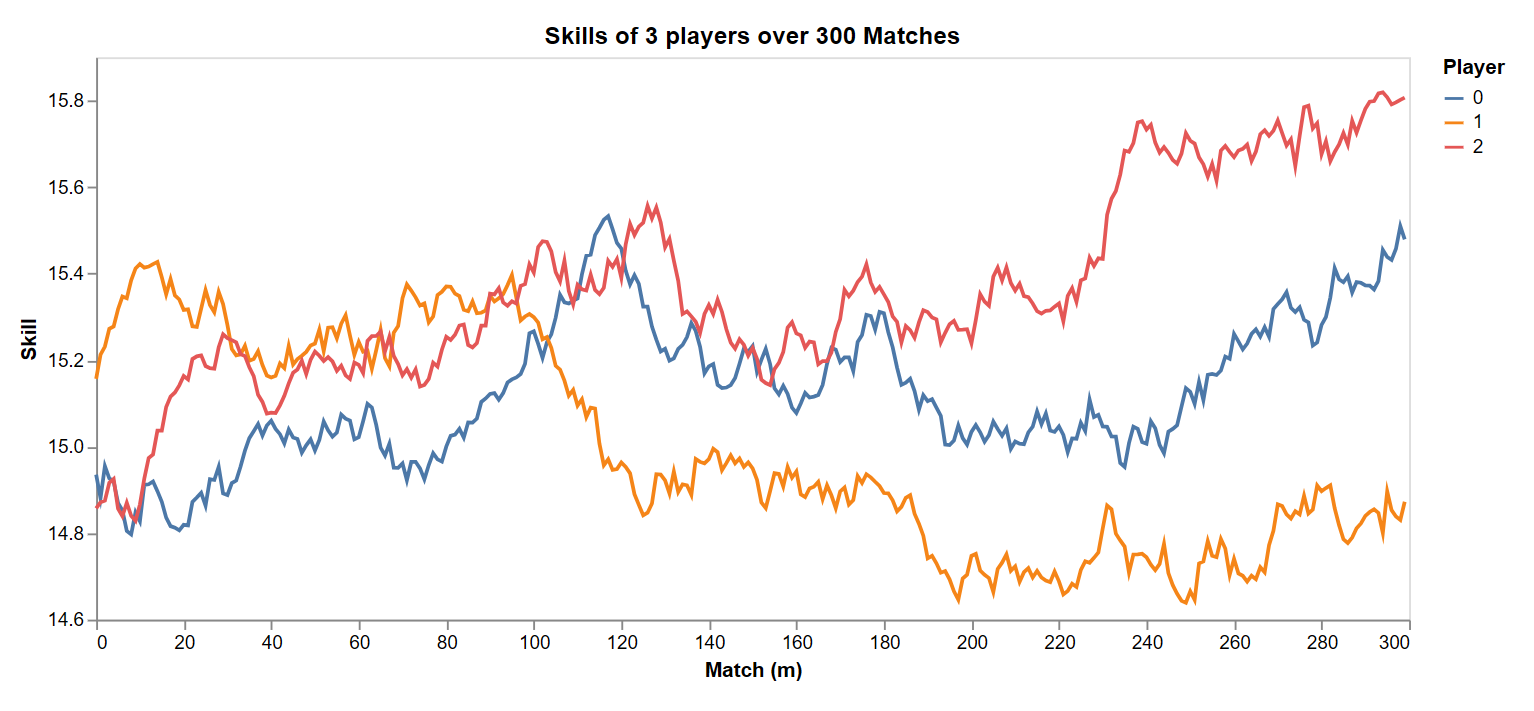
<p>Next, we assume players skill evolve as random gaussian walks over the matches. With three players, that looks like:</p>

<p class="center"><img src="https://duane321.github.io/assets/images/posts/trueskill/skill_over_time.png" alt="Skills Over Time" style="width: 90%" loading="lazy" />
<span class="figure-caption">The match index \(m\) acts like a time index, where we assume there is one match per day involving all players. In this case, skills of three players evolve like a gaussian random walk.</span></p>

<p>This can be expressed as \(s_{i, m+1} \sim \mathcal{N}(s_{i, m}, \gamma^2)\), where \(s_{i, m}\) is player \(i\)’s skill at match \(m\) and \(\gamma\) is a parameter of the simulation, giving the standard deviation of skill change with each match.</p>

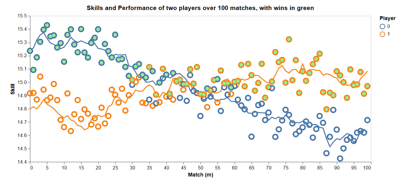
<p>The match outcome is simulated as follows. \(p_{i, m}\) is player \(i\)’s <em>performance</em> on match \(m\) and is normally distributed around their skill. That is, \(p_{i, m} \sim \mathcal{N}(s_{i, m}, \beta^2)\). The standard deviation of performance, \(\beta\), indicates the game’s noisiness. Poker, with its element of chance, has a higher \(\beta\) than chess. For two players and a game without draws, their performances are normally distributed about their skills and the winner, denoted with a green dot, has the higher performance.</p>

<p class="center"><img src="https://duane321.github.io/assets/images/posts/trueskill/performances_of_2.png" alt="Skills and performances" style="width: 90%" loading="lazy" />
<span class="figure-caption">Performances, indicated as circles, are normally distributed, centered on player skill. In this two player game without draws, the player with the higher performance wins, indicated with a green dot.</span></p>

<p>In the style of Elo, the probability of a win for player 1 on match \(m\) is:</p>

\[\Phi\Big(\frac{s_{1, m} - s_{1, m}}{\sqrt{2}\beta}\Big)\]

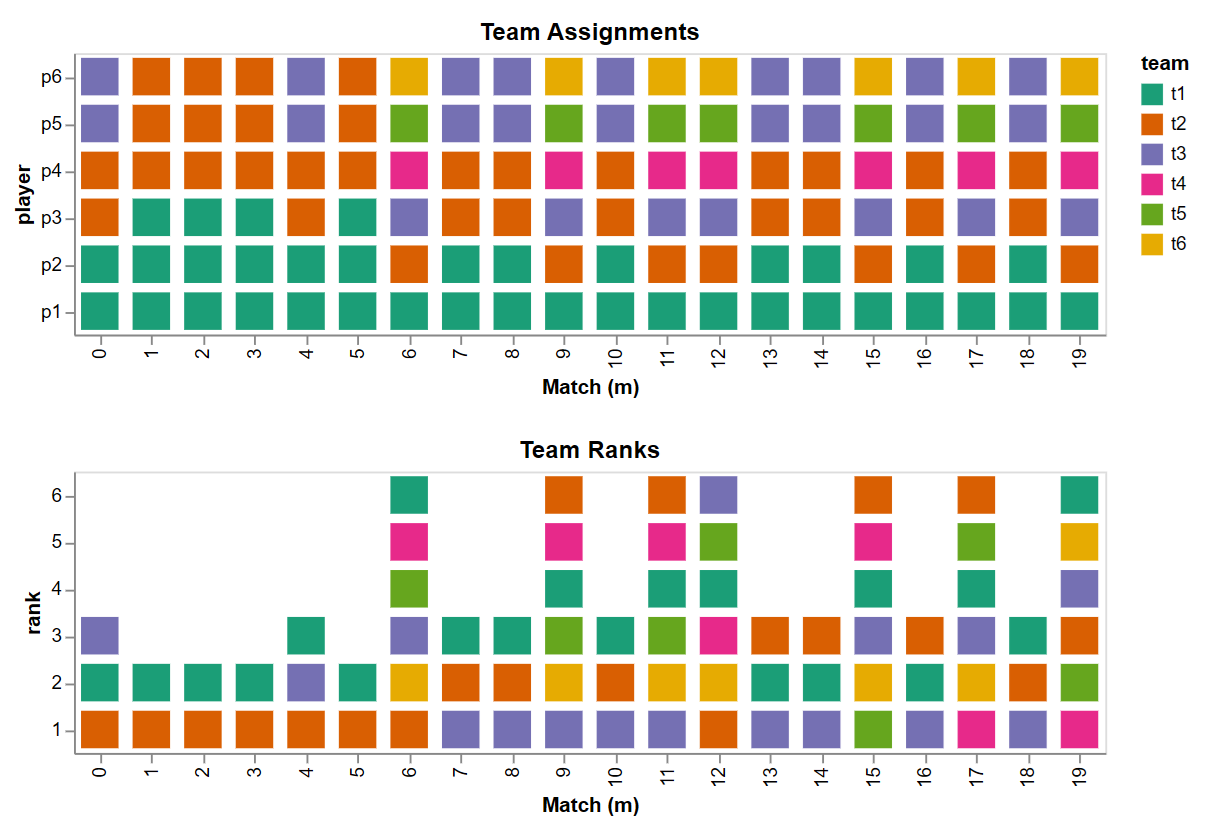
<p>However, unlike Elo, TrueSkill can handle teams. To do this, it assumes the performance of the team is the sum of its players’ performances. If there were \(N=6\) players with three teams of two, then:</p>

\[\begin{align}
t_{1, m} &amp;= p_{1, m} + p_{2, m}\\
t_{2, m} &amp;= p_{3, m} + p_{4, m}\\
t_{3, m} &amp;= p_{5, m} + p_{6, m}
\end{align}\]

<p>In this case, the team with the highest performance wins. Similar to the two player case, the probability that team 1 ranks above team 2 in match \(m\) is:</p>

\[\Phi\Big(\frac{(s_{1, m} + s_{2, m}) - (s_{3, m} + s_{4, m})}{\sqrt{2}\beta}\Big)\]

<p>It should be noted that in multi-team matches, the outcome is not binary; it is a <em>ranking</em> of teams. In a three team match, a match outcome might be \(2, 3, 1\), showing team \(2\) came in first and team \(1\) came in last. These rankings and which players are on which teams constitution the observations; we know their values when applying TrueSkill. Picture that like this:</p>

<p class="center"><img src="https://duane321.github.io/assets/images/posts/trueskill/observations.png" alt="Observations" style="width: 100%" />
<span class="figure-caption">The top plot shows which team each player is on for every match. The bottom plot shows the team rankings for every match.</span></p>

<p>Using only the data shown here, TrueSkill infers players skills and provides uncertainties, quantifying the inference quality.</p>

<p>Seeing this inference is what is enabled by our simulation. We can feed TrueSkill the generated observations, pull out skill estimates and their uncertainties, and compare them to the simulated skills. For one player, we get:</p>

<p class="center"><img src="https://duane321.github.io/assets/images/posts/trueskill/skill_inferred.png" alt="Observations" style="width: 100%" loading="lazy" />
<span class="figure-caption">For a player, TrueSkill infers their skill from the match outcomes. </span></p>

<p>This gives the spirit of TrueSkill, but to show this, a cheat was necessary. Methods like this run into the problem of <em>identifiability</em>; skills cannot be uniquely inferred from observations. One reason is that the probability of a match outcome depends only on skill <em>differences</em>, and there is a whole range of skill pairs with a given skill difference<sup id="fnref:2"><a href="#fn:2" class="footnote" rel="footnote" role="doc-noteref">2</a></sup>. So to create this satisfying recovering-of-the-truth, I allowed TrueSkill to know the actual skill of one player. This anchored the other estimates.</p>

<p>In applied cases, identifiability is not an issue for TrueSkill. It is anchored to match outcome probabilities, and those are the essential ingredients to matchmaking and the primary counterfactual question. In other words, we only care about skill differences and those can be uniquely determined.</p>

<h2 id="trueskill-how-it-works">TrueSkill: How It Works</h2>

<p>The math is sophisticated and detailed, so I will go just deep enough to capture the basics. We will follow the presentation of <a href="https://www.microsoft.com/en-us/research/publication/trueskilltm-a-bayesian-skill-rating-system/" target="_blank" rel="noopener noreferrer">Herbrich et al. (2007)</a>, and explain the computation of a single match, ignoring the random walk of skills over matches. If \(\mathbf{s}\) is a vector of player skills for a match, the goal is to compute its posterior distribution given the observation. That is, we want:</p>

\[p(\mathbf{s} \vert \mathbf{r}, A)\]

<p>where \(A\) tells us which players are on which teams and \(\mathbf{r}\) is the team rankings. Ultimately, we won’t be concerned with the full joint distribution over \(\mathbf{s}\). Rather, we will model each \(s_i\) with a normal distribution, where its mean and variance are the skill estimate and uncertainty we seek. This skill distribution for player \(i\) will be conditional on \(\mathbf{r}\) and \(A\), <em>and</em> on the estimates of the other players.</p>

<p>The example considered has player 1 on team 1, players 2 and 3 on team 2 and player 4 on team 3. The rankings are \((1, 2, 2)\); team 1 came in first and teams 2 and 3 tied for second. We have thus far avoided ties, but these are supported in TrueSkill. Teams tie when their performance is within some small difference \(\epsilon\). In this case, \(\vert t_2  - t_3 \vert &lt; \epsilon\).</p>

<p>To compute the posterior over skills, we must integrate out all possible performances, for both teams and players. Written out explicitly, \(p(\mathbf{s} \vert \mathbf{r}, A)\) is equal to the follow integral:</p>

\[\small
\int_\infty^\infty \int_\infty^\infty \int_\infty^\infty \int_\infty^\infty \int_\infty^\infty \int_\infty^\infty \int_\infty^\infty p(\mathbf{s}, p_1, p_2, p_3, p_4, t_1, t_2, t_3 \vert \mathbf{r}, A)dp_1dp_2dp_3dp_4dt_1dt_2dt_3\]

<p>In this generic form, this is not an easy calculation, even for a single match. However, we can exploit structure in the TrueSkill assumptions for efficiency.</p>

<p>To see this, we start with computing the integrand, more compactly expressed as \(p(\mathbf{s}, \mathbf{p}, \mathbf{t} \vert \mathbf{r}, A)\). This computation is represented with Figure 1 from <a href="https://www.microsoft.com/en-us/research/publication/trueskilltm-a-bayesian-skill-rating-system/" target="_blank" rel="noopener noreferrer">Herbrich et al. (2007)</a>, copied here:</p>

<p class="center"><img src="https://duane321.github.io/assets/images/posts/trueskill/figure_1_from_original_paper.png" alt="illustration" style="width: 100%" />
<span class="figure-caption">This is a factor graph representing the computation of \(p(\mathbf{s}, \mathbf{p}, \mathbf{t} \vert \mathbf{r}, A)\) under the TrueSkill data generation assumptions.</span></p>

<p>This is a <em>factor graph</em> representation of \(p(\mathbf{s}, \mathbf{p}, \mathbf{t} \vert \mathbf{r}, A)\), where \(\mathbf{r}=(1,2,2)\) and \(A\) represents the team participations, as described. To be clear, \(\mathbf{r}\) and \(A\) dictate the shape of the graph. Just like \(p(\mathbf{s}, \mathbf{p}, \mathbf{t} \vert \mathbf{r}, A)\), think of this graph as something that receives values of \(\mathbf{s}, \mathbf{p}, \mathbf{t}\) and gives back a number. Though it is more than that, as we’ll see.</p>

<p>Computing \(p(\mathbf{s}, \mathbf{p}, \mathbf{t} \vert \mathbf{r}, A)\) involves a product of <em>factors</em>, which are functions of variables. To understand this, we explain the factor graph.</p>

<p>A factor graph has two types of nodes. Large circles (so not including the small numbered circles) represent random variables. The first row of circle nodes labeled \(s_1, \cdots, s_4\) are the player skills as of this match. The second row, labeled \(p_1, \cdots, p_4\) are player performances. The third row, labeled, \(t_1, t_2, t_3\) are team performances. The last row gives rank-consecutive team performance differences. That is, \(d_1 = t_1 - t_2\) and \(d_2 = t_2 - t_3\). As will be discussed next, these variables are introduced to assert the given \(\mathbf{p}\) and \(\mathbf{t}\) are consistent with \(\mathbf{r} = (1,2,2)\).</p>

<p>Black square nodes represent factors, functions of those random variables that connect with them. So the top row of black squares are four functions of \(s_1, s_2, s_3, s_4\) respectively. In fact, they are normal densities under \(\mu_i\) and \(\sigma_i\), representing their prior distributions (or distributions conditional on previous matches). The next row of black squares represent the densities of performances given skills and \(\beta\). The third row of black squares are indicator functions checking whether the team performances in fact sum to the player performances. This is to zero-out combinations of \(\mathbf{p}\) and \(\mathbf{t}\) that don’t match that definition. The second to last row and last row define \(d_1\) and \(d_2\) and indicate whether they are such to produce the \(\mathbf{r}=(1,2,2)\) ranking.</p>

<p>The factor graph instructs a faster computation than the generic six-nested integral. This is because each factor only concerns a small subset of variables, those connected to it. Put simply, given \(\mathbf{s}, \mathbf{p}, \mathbf{t}\), we could compute products of factors, starting from the top black squares and cascading downwards, producing a number equal to \(p(\mathbf{s}, \mathbf{p}, \mathbf{t} \vert \mathbf{r}, A)\). If the given \(\mathbf{s}\), \(\mathbf{p}\) and \(\mathbf{t}\) were inconsistent with \(\mathbf{r}\) and \(A\), the result is zero. That is the purpose of the indicator functions seen in the graph.</p>

<p>What remains is to integrate out \(\mathbf{p}\) and \(\mathbf{t}\) from \(p(\mathbf{s}, \mathbf{p}, \mathbf{t} \vert \mathbf{r}, A)\). This is done with <em>Expectation Propagation</em> (EP), a message passing algorithm from the category of <em>variational inference</em> methods. This is an extensive topic, so I will be brief. Essentially, the integration can be <em>approximated</em> with an iterative but fast computation that proceeds down and up the graph, as indicated with light-to-dark curved arrows. The messages flowing through the graph all take the form of univariate normal distributions, even for the non-gaussian portions of the graph near the indicator functions. Gaussians are chosen because they make products and integrals easy.</p>

<p>For some intuition on variational methods, see <a href="/concepts/probabilistic-graphical-models/pgms-part-3/" target="_blank" rel="noopener noreferrer">Part 3 of my series on Probabilistic Graphical Models</a>. For a more complete explanation, see <a href="https://www.microsoft.com/en-us/research/publication/trueskilltm-a-bayesian-skill-rating-system/" target="_blank" rel="noopener noreferrer">Herbrich et al. (2007)</a> or section 22.5 of <a href="https://probml.github.io/pml-book/book0.html" target="_blank" rel="noopener noreferrer">Murphy (2012)</a>.</p>

<p>The point is we can approximate the integral with an efficient computation over this graph, made possible by the TrueSkill assumptions and the EP algorithm. Further, it is simply combined with the random walk of skills over matches; the same up-down routine can be used to update skill estimates with each new match.</p>

<p>Doing so provides a univariate distribution over each player \(i\)’s skill \(s_i\), with mean \(\hat{\mu}_i\) and standard deviation \(\hat{\sigma}_i\). These values represent not only who a player has beaten, but who the beaten player has beaten, and so on, for all chains of matches. Naturally, these skills are used to rank players. For XBox Live, players were ranked according to a conservative skill estimate of \(\hat{\mu}_i - 3\hat{\sigma}_i\).</p>

<p>Most importantly, given any two players, including those who have never played each other, we can accurately estimate the probability of a win or loss.</p>

<h2 id="trueskill-performance">TrueSkill Performance</h2>

<p>In <a href="https://www.microsoft.com/en-us/research/publication/trueskilltm-a-bayesian-skill-rating-system/" target="_blank" rel="noopener noreferrer">Herbrich et al. (2007)</a>, there are several quantifications and plots demonstrating TrueSkill’s efficacy. One that I found especially convincing is copied here:</p>

<p class="center"><img src="https://duane321.github.io/assets/images/posts/trueskill/delta_from_50.png" alt="Performance Graph" style="width: 60%" />
<span class="figure-caption">An optimal matchmaking system will ensure one-on-one games have close to a 50% probability of player 1 winning. However, in real applications, it takes some games for the system to determine skill levels, to make those 50-50 matches. For each skill measure, this skill plot shows the difference from 50% of the empirical win-rate. A value of 0 is optimal. This plot shows that TrueSkill is closer to 0 and approaches it more quickly then Elo or the Halo 2 ranking system.</span></p>

<h2 id="trueskill-variants">TrueSkill Variants</h2>

<p>Since TrueSkill’s publishing, there have been several notable extensions:</p>

<ul>
  <li>
    <p><strong>TrueSkill Through Time</strong> (<a href="https://www.microsoft.com/en-us/research/publication/trueskill-through-time-revisiting-the-history-of-chess/" target="_blank" rel="noopener noreferrer">Dangauthier (2008)</a>): An interesting limitation of vanilla TrueSkill is that skill estimates depend only on past matches. However, suppose a player defeated someone who later became the champion. In retrospect, the estimate of the player who beat the champion should be revised upward. This is the difference between vanilla TrueSkill, performing <em>filtering,</em> and TrueSkill Through Time, performing <em>smoothing</em>. Smoothing is the better option for retroactively determining the GOAT.</p>

    <p>Another element is that vanilla TrueSkill assumptions skills only change with matches. TrueSkill Through Time assumes skills evolve over time. This is more realistic, since it is likely that matches occur outside of the data or skills change due other time related factors, like age.</p>
  </li>
  <li>
    <p><strong>TrueSkill 2</strong> (<a href="https://www.microsoft.com/en-us/research/publication/trueskill-2-improved-bayesian-skill-rating-system/?msockid=0749eb24e7c9612828c2f976e67c6045" target="_blank" rel="noopener noreferrer">Minka (2018)</a>): Vanilla TrueSkill only operates on wins, losses and draws, but in most games, there’s other useful information. TrueSkill 2 is an extension to factor in, among other things, players quitting matches, death/kill ratios, and correlations across match types.</p>
  </li>
  <li>
    <p><strong>Multidimensional Skill</strong> (<a href="https://doi.org/10.1145/2835776.2835787" target="_blank" rel="noopener noreferrer">Chen (2016)</a>): While not a TrueSkill variant, it is worth mentioning. An assumption of TrueSkill is that a skill is a single number. However, players and their styles might not be so simply modeled. We could have an arrangement like rock-paper-scissors, where player 1 has an advantage of player 2, who has an advantage of player 3, who has an advantage of player 1. This presents <em>intransitivity</em>; observing player 1 beating player 2 many times and player 2 beating player 3 many times may not be enough to confidently say player 1 will beat player 3. It should be noted that this is an exotic effect to capture, and most systems consider univariate skills.</p>
  </li>
</ul>

<h2 id="the-details">The Details</h2>

<p>For those interested in the details of the above analysis, see <a href="https://github.com/Duane321/true_theta/blob/main/posts/trueskill/true_skill_simulated.ipynb" target="_blank" rel="noopener noreferrer">this notebook</a>. It relies on the <a href="https://trueskill.org/" target="_blank" rel="noopener noreferrer">TrueSkill implementation</a> by <a href="https://subl.ee/" target="_blank" rel="noopener noreferrer">Heungsub Lee</a>.</p>

<h2 id="part-two">Part Two</h2>

<p>We have briefly toured the ingenious TrueSkill algorithm, but we’ve yet to see it applied to real data. In an upcoming post, we will apply it to boxing, tennis and warcraft 3, a classic real time strategy game.</p>

<hr />
<h3 id="references">References</h3>

<ol>
  <li>
    <p>R. Herbrich, T. Minka, T. Graepel. <a href="https://www.microsoft.com/en-us/research/publication/trueskilltm-a-bayesian-skill-rating-system/" target="_blank" rel="noopener noreferrer">TrueSkill(TM): A Bayesian Skill Rating System</a> Advances in Neural Information Processing Systems. January 2007</p>
  </li>
  <li>
    <p>P. Dangauthier, R. Herbrich, T. Minka, T. Graepel. <a href="https://www.microsoft.com/en-us/research/publication/trueskill-through-time-revisiting-the-history-of-chess/" target="_blank" rel="noopener noreferrer">TrueSkill Through Time: Revisiting the History of Chess</a> In Advances in Neural Information Processing Systems. MIT Press, January 2008</p>
  </li>
  <li>
    <p>T. Minka, R. Cleven, Y. Zaykov. <a href="https://www.microsoft.com/en-us/research/publication/trueskill-2-improved-bayesian-skill-rating-system/?msockid=0749eb24e7c9612828c2f976e67c6045">TrueSkill 2: An improved Bayesian skill rating system</a>. Microsoft. March 2018</p>
  </li>
  <li>
    <p>S. Chen, T. Joachims. <a href="https://doi.org/10.1145/2835776.2835787" target="_blank" rel="noopener noreferrer">Modeling Intransitivity in Matchup and Comparison Data</a> Association for Computing Machinery. 2016</p>
  </li>
  <li>
    <p>K. Murphy. <a href="https://probml.github.io/pml-book/book0.html" target="_blank" rel="noopener noreferrer">Machine Learning: A Probabilistic Perspective</a>. <em>MIT Press</em>. 2012.</p>
  </li>
</ol>

<hr />
<h3 id="footnotes">Footnotes</h3>

<div class="footnotes" role="doc-endnotes">
  <ol>
    <li id="fn:1">
      <p>In practice, the ELO system is slightly different. Beta is used to scale skills to be in the range of a few thousand. Also, the logistic function, rather than the normal CDF, is used for compute purposes. <a href="#fnref:1" class="reversefootnote" role="doc-backlink">&#8617;</a></p>
    </li>
    <li id="fn:2">
      <p>Some of this is relieved with a prior distribution over skills, but that only mitigates the issue. For instance, if one player <em>always</em> beats another player, then there is a huge range of plausible skill pairs. They need only have at least some large skill difference. A prior will bias this difference to be smaller, but the truth of the matter may be a much larger difference. <a href="#fnref:2" class="reversefootnote" role="doc-backlink">&#8617;</a></p>
    </li>
  </ol>
</div>]]></content><author><name>Duane Rich</name></author><category term="machine-learning-and-other-topics" /><category term="Post Formats" /><summary type="html"><![CDATA[A walkthrough of the classic, effective and beautiful TrueSkill algorithm.]]></summary><media:thumbnail xmlns:media="http://search.yahoo.com/mrss/" url="https://duane321.github.io/assets/images/posts/trueskill/figure_1_from_original_paper.png" /><media:content medium="image" url="https://duane321.github.io/assets/images/posts/trueskill/figure_1_from_original_paper.png" xmlns:media="http://search.yahoo.com/mrss/" /></entry><entry><title type="html">MLflow</title><link href="https://duane321.github.io/concepts/ai-tool-reviews/mlflow/" rel="alternate" type="text/html" title="MLflow" /><published>2025-02-02T00:00:00+00:00</published><updated>2025-02-02T00:00:00+00:00</updated><id>https://duane321.github.io/concepts/ai-tool-reviews/mlflow</id><content type="html" xml:base="https://duane321.github.io/concepts/ai-tool-reviews/mlflow/"><![CDATA[<p>In this article, we’ll review <a href="https://mlflow.org/" target="_blank" rel="noopener noreferrer">MLflow</a>, an open source tool for easing the management of machine learning models. At the end, we’ll provide a one page PDF summarizing our take.</p>

<h2 id="mlflow-tracking">MLflow Tracking</h2>

<p>MLflow addresses a common circumstance of data scientists. They are experimenting with a model (e.g. adjusting its hyperparameters, changing the preprocessing, updating the data) to get good performance. The annoyance is that these experiments are distributed across space (e.g. using multiple notebooks) and time (e.g. changing hyperparameters within the same notebook), and that makes finding the best model difficult. A disciplined scientist will collect all experiments into one place for comparability, but this is an additional, manual and unreliable workflow.</p>

<p>MLflow’s solution is to provide a UI which displays these experiments. To do this, a user needs only to update their model training code with a few API calls. Specifically, a user wraps their model training code within <code class="language-plaintext highlighter-rouge">mlfow.start_run()</code> and <code class="language-plaintext highlighter-rouge">.log_params</code>-the values they wish to compare across experiments:</p>

<div class="language-python highlighter-rouge"><div class="highlight"><pre class="highlight"><code><span class="n">mlflow</span><span class="p">.</span><span class="nf">set_experiment</span><span class="p">(</span><span class="sh">"</span><span class="s">experiment_1</span><span class="sh">"</span><span class="p">)</span>

<span class="k">with</span> <span class="n">mlflow</span><span class="p">.</span><span class="nf">start_run</span><span class="p">():</span>
  <span class="n">mlf</span><span class="p">.</span><span class="nf">log_param</span><span class="p">(</span><span class="sh">"</span><span class="s">lr</span><span class="sh">"</span><span class="p">,</span> <span class="mf">0.001</span><span class="p">)</span>
  <span class="c1"># Model training code goes here
</span>  <span class="n">mlf</span><span class="p">.</span><span class="nf">log_param</span><span class="p">(</span><span class="sh">"</span><span class="s">loss</span><span class="sh">"</span><span class="p">,</span> <span class="n">loss</span><span class="p">)</span>
</code></pre></div></div>

<p>Every time this code block executes, the parameter <code class="language-plaintext highlighter-rouge">lr</code> and the resulting performance <code class="language-plaintext highlighter-rouge">loss</code> are logged and made available via an UI, accessible with the following CLI command:</p>

<div class="language-plaintext highlighter-rouge"><div class="highlight"><pre class="highlight"><code>mlflow ui --port 5000
</code></pre></div></div>

<p>Giving something like:</p>

<p class="center"><img src="https://duane321.github.io/assets/images/posts/ai_tool_review/mlflow/mlflow_screenshot.png" alt="illustration" style="width: 100%" /></p>

<p>Alternatively, <a href="https://mlflow.org/docs/latest/tracking.html#tracking-server" target="_blank" rel="noopener noreferrer">remote experimental tracking</a> is available, so multiple people develop on the same model.</p>

<p>What we’ve done is provide a very brief description of <strong>MLflow Tracking</strong>. The other core components that caught our attention were <strong>MLflow Models</strong>, <strong>MLflow Projects</strong> and the <strong>MLflow Registry</strong>.</p>

<h2 id="mlflow-models">MLflow Models</h2>

<p>For portability (something essential for production ML), MLflow provides model standardization. They provide methods which convert a variety of models (e.g. sklearn, pytorch, etc.) into their standard format<sup id="fnref:1"><a href="#fn:1" class="footnote" rel="footnote" role="doc-noteref">1</a></sup>, which can then be loaded and/or served in different environments, such as Docker, Apache Spark, AWS SageMaker, and Azure ML.</p>

<p>To support this, MLflow offers ‘flavors’, model abstractions that permit execution in different environments. Some example flavors are <code class="language-plaintext highlighter-rouge">python_function</code>, <code class="language-plaintext highlighter-rouge">sklearn</code>, <code class="language-plaintext highlighter-rouge">pytorch</code>, and <code class="language-plaintext highlighter-rouge">onnx.</code> These allow models to be saved/loaded in a variety of environments, provide interoperability between ML libraries, support multiple inference methods, and help track dependencies and metadata.</p>

<h2 id="mlflow-projects">MLflow Projects</h2>

<p>To a data scientist, a directory might be their final deliverable. All one needs to do is enter the directory and run a CLI command. For example, that command might pull in the data, train the model, make predictions and store those predictions in a shared database.</p>

<p>For collaboration and reproducibility, MLflow Projects standardizes this practice. That is, it provides a way to package machine learning code so that it can be shared and executed reproducibly and across environments. Essentially, an MLflow Project is a directory containing code structured according to certain conventions. To do this, a central element of MLflow Projects is the <code class="language-plaintext highlighter-rouge">MLproject</code> file, a YAML configuration that defines the project’s entry points (its run commands), dependencies, and execution environment.</p>

<p>Further, MLflow Projects permit multi-step workflows, where different tasks (e.g. data processing, model training, and evaluation) can be orchestrated in a structured pipeline. These workflows can be executed sequentially or in parallel.</p>

<h2 id="mlflow-registry">MLflow Registry</h2>

<p>The MLflow Registry is a centralized model store. It allows teams to track model versions, add descriptions, and assign metadata to models. It’s especially good for collaboration, as individuals can track and contribute to the same ‘champion’ model.</p>

<h2 id="strengths">Strengths</h2>

<p>From our experience and surveying Github issues, reddit threads and other user experience sources, we determine its primary strength:</p>

<ul>
  <li>
    <p><strong>Open source and Active</strong>: As industry applications have grown, the developer community has <a href="https://github.com/mlflow/mlflow/graphs/contributors" target="_blank" rel="noopener noreferrer">only accelerated</a>. Major companies use MLflow, which speaks to its enterprise viability. The documentation is detailed. Github issues are discussed promptly, normally with a solution planned or highlighted. Newer applications, like LLM specific utilities, are feature incomplete but are receiving active attention.</p>
  </li>
  <li>
    <p><strong>Flexible</strong>: A challenge of machine learning model management is supporting the wide and diverse software ecosystem for ML modeling. MLflow has made impressive progress on this task, supporting <a href="https://mlflow.org/docs/latest/models.html#built-in-model-flavors" target="_blank" rel="noopener noreferrer">a complex variety of models</a>. Github issues suggest LLM support is incomplete, but this is receiving active attention (e.g. they recently announced an <a href="https://mlflow.org/docs/latest/llms/llama-index/index.html#why-use-llamaindex-with-mlflow" target="_blank" rel="noopener noreferrer">integration with LLamaIndex</a>).</p>
  </li>
  <li>
    <p><strong>Minimalistic</strong>: MLflow understands that frequent calls to their API is a bad thing. Since many workflows are common (e.g. training a scikit-learn model), their methods offer sensible defaults, requiring less user specification, and they offer the <code class="language-plaintext highlighter-rouge">auto_log</code> method, which allows users to avoid making logging calls.</p>
  </li>
  <li>
    <p><strong>Intuitive</strong>: Their UI for tracking and viewing experiments is intuitive. In our opinion, they provide plots of the most typical views of experimental results. That said, users have complained about UI inflexibility. Certain specialized views are not available and require users to code their own visualizations.</p>
  </li>
</ul>

<h2 id="weaknesses">Weaknesses</h2>

<p>Also from our experience and surveying user experiences, we determine its primary weaknesses:</p>

<ul>
  <li>
    <p><strong>DevOp Requirements</strong>: MLflow is self-hosted; it is code that the user runs on their own systems. This is a virtue to some, but it creates an infrastructure management burden, which does not exist with fully managed alternatives, like Weights &amp; Biases. For this reason, MLflow is more appropriate for companies staffed with this expertise.</p>
  </li>
  <li>
    <p><strong>Lock-in</strong>: MLflow offers a managed alternative, <a href="https://www.databricks.com/product/managed-mlflow" target="_blank" rel="noopener noreferrer">Managed MLflow</a> by Databricks. This essentially outsources the infrastructure work to Databricks, which has added benefits (e.g. it can serve a user’s model via an API), but also has downsides. The fixed cost of migration can be high and the variable costs of running jobs can be high. Further, it creates lock-in going forward; once integrated, future database migrations are notoriously challenging.</p>
  </li>
  <li>
    <p><strong>Scaling</strong>: For the largest applications, we’ve heard complaints of MLflow’s sluggishness and insufficient support for distributed training and scaled ETL jobs. Managing a massive amount of artifacts (data produced during training) or parameters can create slow API calls and a lagged UI. Further, MLflow was not originally developed for scaled applications. Dedicated alternatives, which offer MLflow-like tracking, are often preferred in such cases.</p>
  </li>
</ul>

<h2 id="summary">Summary</h2>

<p>To make this discussion portable, we’ve packaged the main points into a downloadable PDF:</p>

<div class="pdf_pc">
	<object data="/assets/images/posts/ai_tool_review/mlflow/mlflow.pdf" type="application/pdf" width="100%" height="110%" style="border: none; max-width: 100%; margin-left: auto; margin-right: auto;">
		<iframe src="/assets/images/posts/ai_tool_review/mlflow/mlflow.pdf" type="application/pdf" width="100%" height="110%" style="border: none; max-width: 100%; margin-left: auto; margin-right: auto;">
	</iframe>
	<p>
		Your browser does not support PDFs.
		<a href="/assets/images/posts/ai_tool_review/mlflow/mlflow.pdf" download="">Download the PDF</a>.
	</p>
	</object>
</div>

<div class="pdf_mobile">
	<div class="mobile_pdf_placeholder">
		<img src="/assets/images/posts/ai_tool_review/mlflow/mlflow_pdf_placeholder.png" alt="PDF" />
	</div>
</div>

<p><a href="/assets/images/posts/ai_tool_review/mlflow/mlflow.pdf" download="" class="pdf_download_button">Download PDF</a></p>

<hr />
<h3 id="footnotes">Footnotes</h3>

<div class="footnotes" role="doc-endnotes">
  <ol>
    <li id="fn:1">
      <p>The <a href="https://mlflow.org/docs/latest/models.html#id13" target="_blank" rel="noopener noreferrer">format</a> is a directory of files, containing an <code class="language-plaintext highlighter-rouge">MLmodel</code> file. <a href="#fnref:1" class="reversefootnote" role="doc-backlink">&#8617;</a></p>
    </li>
  </ol>
</div>]]></content><author><name>DJ Rich</name></author><category term="ai-tool-reviews" /><category term="Post Formats" /><summary type="html"><![CDATA[A one page review of MLflow, the ML model management platform.]]></summary><media:thumbnail xmlns:media="http://search.yahoo.com/mrss/" url="https://duane321.github.io/assets/images/posts/ai_tool_review/mlflow/mlflow_logo.png" /><media:content medium="image" url="https://duane321.github.io/assets/images/posts/ai_tool_review/mlflow/mlflow_logo.png" xmlns:media="http://search.yahoo.com/mrss/" /></entry><entry><title type="html">Ray</title><link href="https://duane321.github.io/concepts/ai-tool-reviews/ray/" rel="alternate" type="text/html" title="Ray" /><published>2025-01-26T00:00:00+00:00</published><updated>2025-01-26T00:00:00+00:00</updated><id>https://duane321.github.io/concepts/ai-tool-reviews/ray</id><content type="html" xml:base="https://duane321.github.io/concepts/ai-tool-reviews/ray/"><![CDATA[<p>Keeping track of publicly available technology is an important part of honest machine learning consulting. Almost always, the best solution for a client is <em>not</em> for the consultant to build from scratch. In fact, an informed client should be suspicious of such a recommendation. Primarily, the consultant’s role is to build software connecting powerful tools to the specific operations of the client<sup id="fnref:1"><a href="#fn:1" class="footnote" rel="footnote" role="doc-noteref">1</a></sup>.</p>

<p>So we pay close attention to the AI/ML landscape.</p>

<h1 id="ray">Ray</h1>

<p>A growing tool is Ray, the AI computing framework. It’s finding its place among leading companies in AI/ML applications:</p>

<ul>
  <li><a href="https://www.uber.com/blog/how-uber-uses-ray-to-optimize-the-rides-business/" target="_blank" rel="noopener noreferrer">Uber used it</a> for strong market optimization improvements and a boost to developer productivity.</li>
  <li><a href="https://tech.instacart.com/distributed-machine-learning-at-instacart-4b11d7569423" target="_blank" rel="noopener noreferrer">Instacart used it</a> to improve resource utilization, developer productivity and reduced execution time.</li>
  <li><a href="https://medium.com/pinterest-engineering/last-mile-data-processing-with-ray-629affbf34ff" target="_blank" rel="noopener noreferrer">Pinterest used it</a> to see similar gains.</li>
</ul>

<p>This inspired us to get familiar with RAY, survey the positive and negative<sup id="fnref:2"><a href="#fn:2" class="footnote" rel="footnote" role="doc-noteref">2</a></sup> use cases, and clean up our understanding into a shareable one pager:</p>

<div class="pdf_pc">
	<object data="/assets/images/posts/ai_tool_review/ray/RAY.pdf" type="application/pdf" width="100%" height="110%" style="border: none; max-width: 100%; margin-left: auto; margin-right: auto;">
		<iframe src="/assets/images/posts/ai_tool_review/ray/RAY.pdf" type="application/pdf" width="100%" height="110%" style="border: none; max-width: 100%; margin-left: auto; margin-right: auto;">
	</iframe>
	<p>
		Your browser does not support PDFs.
		<a href="/assets/images/posts/ai_tool_review/ray/RAY.pdf" download="">Download the PDF</a>.
	</p>
	</object>
</div>

<div class="pdf_mobile">
	<div class="mobile_pdf_placeholder">
		<img src="/assets/images/posts/ai_tool_review/ray/RAY_PDF_placeholder.png" alt="PDF" />
	</div>
</div>

<p><a href="/assets/images/posts/ai_tool_review/ray/RAY.pdf" download="" class="pdf_download_button">Download PDF</a></p>

<hr />
<h3 id="footnotes">Footnotes</h3>

<div class="footnotes" role="doc-endnotes">
  <ol>
    <li id="fn:1">
      <p>In fact, this makes for no shortage of work. We often observe clients’ asks to be so specialized, no publicly available, designed-for-growth product quite does the trick. <a href="#fnref:1" class="reversefootnote" role="doc-backlink">&#8617;</a></p>
    </li>
    <li id="fn:2">
      <p>Few publicly express what failed, so we rely on our own experience, word of mouth and public discussions (X, reddit and GitHub issues mostly). <a href="#fnref:2" class="reversefootnote" role="doc-backlink">&#8617;</a></p>
    </li>
  </ol>
</div>]]></content><author><name>DJ Rich</name></author><category term="ai-tool-reviews" /><category term="Post Formats" /><summary type="html"><![CDATA[A one page review of Ray, the AI computing framework.]]></summary><media:thumbnail xmlns:media="http://search.yahoo.com/mrss/" url="https://duane321.github.io/assets/images/posts/ai_tool_review/ray/ray_logo.png" /><media:content medium="image" url="https://duane321.github.io/assets/images/posts/ai_tool_review/ray/ray_logo.png" xmlns:media="http://search.yahoo.com/mrss/" /></entry><entry><title type="html">Algorithmic Operations: Lessons from Bandit Algorithms</title><link href="https://duane321.github.io/concepts/machine-learning-and-other-topics/algorithmic-operations/" rel="alternate" type="text/html" title="Algorithmic Operations: Lessons from Bandit Algorithms" /><published>2024-11-18T00:00:00+00:00</published><updated>2024-12-10T00:00:00+00:00</updated><id>https://duane321.github.io/concepts/machine-learning-and-other-topics/algorithmic-operations</id><content type="html" xml:base="https://duane321.github.io/concepts/machine-learning-and-other-topics/algorithmic-operations/"><![CDATA[<blockquote>
  <p><span style="color:#205081"><strong>Algorithmic Operations</strong></span>: the maximal use of algorithms to make essential business decisions.</p>
</blockquote>

<p>The practice can be traced to the hedge fund industry. The operations of ingesting data to predict prices and execute trades is a friendly environment to algorithms, which are constrained to act only via programmatic interfaces. By the mid 1990’s, the early-digitized financial markets produced decisive proof of algorithms’ efficacy in the form of the unprecedented success of quantitative hedge funds like Renaissance Technologies and D. E. Shaw. Its influence spread, with one path traceable from D. E. Shaw, when Jeff Bezos, a freshly indoctrinated algorithm evangelist, left the company to start Amazon in 1994.</p>

<p>However, the retail business lacked programmatic access. In the late 1990’s, ordering from wholesalers, tracking shipments, directing inventory, packaging items, and shipping orders were frequently done manually. Ordering from wholesalers often involved phone calls or faxed purchase orders, tracking shipments relied on manually updated spreadsheets or physical ledgers, inventory management required store managers to walk through aisles with clipboards, and packaging and shipping orders depended on workers assembling boxes with printed labels based on handwritten instructions. To direct these operations digitally would require new technology throughout the entire supply chain. Over the following three decades, Amazon performed this transformation with enormous effort and contributed<sup id="fnref:1"><a href="#fn:1" class="footnote" rel="footnote" role="doc-noteref">1</a></sup> to a growing industry philosophy of algorithmic essentialism.</p>

<p>Today, entire industries, like ridesharing, depend sensitively on effective algorithmic operations and any declaration of its value reads as a cliché. Yet, they remain the exception rather than the norm. Recognizing colloquialisms like ‘Excel Hell’, ‘Email Ping-Pong’ and ‘Death by Meeting’ is all one needs to appreciate this fact. The answer to ‘why?’ is ‘because it is hard’. This article seeks to explore this more thoroughly.</p>

<p>More constructively, this article is to provide clarity on the causes and make informed recommendations for progress. In total, this is an article about automated decisioning.</p>

<p>Our approach is to compare a company’s algorithmic operations to those of fully programmatic learning algorithms. The analogy contextualizes problems and clarifies requirements. Further, in our recommendations, we cite time-tested, nonspeculative solutions.</p>

<p>This article is informed by the authors’ combined 8 years of experience at Lyft, a review of 14 Amazon employee interviews, comments from other industry practitioners, and a survey of literature, including 12 MLOps papers and nearly 100 blogs from Lyft, Uber, Instacart, DoorDash and Airbnb. We focus on these companies because they have been successful in algorithmic operations and are local to our experience.</p>

<h2 id="algo-ops-what-it-is">Algo Ops: What It Is</h2>

<p>Repeating the definition, Algorithmic Operations (‘Algo Ops’) refer to the maximal use of algorithms to make essential business decisions. The term ‘maximal’ is used as an alternative to ‘exclusive’, since no organization exclusively uses algorithms for decisions. This is to suggest ‘getting algorithms to do everything they can and should do.’</p>

<p>Algo Ops are different from algorithmic products. Algo Ops are about automating the internal machinery of a company, while algorithmic products are about delivering value to users through algorithm-driven features. Google Search’s decision of which websites to return most directly benefits the user. Uber’s dynamic pricing system is designed for revenue and profitability. Both rely on  algorithms, but their context, intent and beneficiaries set them apart. These differences create distinct desiderata and challenges.</p>

<p>Algo Ops are different from Machine Learning Operations (‘MLOps’), though they heavily overlap. Indeed, much of our literature review was from MLOps. However, while MLOps focuses on the development lifecycle of ML models<sup id="fnref:2"><a href="#fn:2" class="footnote" rel="footnote" role="doc-noteref">2</a></sup>, Algo Ops encompasses the broader application of algorithms to automate and optimize decision making across the entire business. MLOps is a critical component of Algo Ops, but not all algorithms involved in business operations are ML models. For example, data-less rule-based systems, optimization algorithms, and other non-ML methods are integral parts of Algo Ops. Revealing the term’s breadth, Algo Ops subsumes much of operations research in addition to MLOps.</p>

<p>We’ll also define <em>partial</em> Algo Ops, or Algo Ops designed with ‘humans-in-the-loop.’ Partial Algo Ops, for many categories of decisions, are best practices. An example is the the entire scientific discipline of commercial experimentation, whereby control and treatments groups are deployed, logged and analyzed to inform a person’s go/no-go decision. Partial Algo Ops are accepted as the final destination, since many questions cannot be raised and answered by algorithms alone, like some system-level engineering decisions or UI design choices. Other motivations are for transparency and well defined accountability. Further, they may benefit when difficult-to-measure economic trade-offs are involved, and can only be properly balanced with domain experts. In other cases, partial Algo Ops are considered an intermediate step on the way to Algo Ops; humans are there to ‘fill in the gaps’.</p>

<h2 id="deploy-explore-log-learn">Deploy, Explore, Log, Learn</h2>

<p>In pursuit of Algo Ops, we will consistently reference a framework described in the 2017 Microsoft Research paper “Making Contextual Decisions with Low Technical Debt.” <a href="https://arxiv.org/abs/1606.03966" target="_blank" rel="noopener noreferrer">Agarwal et al. (2017)</a> was partially a response to the well known 2015 Google paper “Hidden Technical Debt in Machine Learning Systems,” which explained the pernicious causes underneath the expensive and deleterious process of large scale machine learning model maintenance. <a href="https://arxiv.org/abs/1606.03966" target="_blank" rel="noopener noreferrer">Agarwal et al. (2017)</a> explains the ‘Deploy, Explore, Log, Learn’ framework (“DELL” as only we will call it) in their presentation of their ‘Decision Service’, a product enabling applications of contextual bandit (CB) algorithms and addressing challenges described in <a href="https://papers.nips.cc/paper_files/paper/2015/hash/86df7dcfd896fcaf2674f757a2463eba-Abstract.html" target="_blank" rel="noopener noreferrer">Sculley et al. (2015)</a>.</p>

<p>Bandit algorithms are of particular interest because they perform the complete loop of automated decisioning, including observing, deciding and learning. They are dedicated to the expansive class of causal modeling, which encapsulates predictive modeling<sup id="fnref:3"><a href="#fn:3" class="footnote" rel="footnote" role="doc-noteref">3</a></sup>. Indeed, bandit algorithms are attractive for this completeness, but such completeness brings the full set of technical issues. The paper’s approach to this broad class of challenges is what makes it relevant for our purposes.</p>

<p><a href="https://arxiv.org/abs/1606.03966" target="_blank" rel="noopener noreferrer">Agarwal et al. (2017)</a> present DELL as a software abstraction designed to capture a wide range of automated decisioning applications. More technically, they recognize that any CB system’s data is be made up of, implicitly or explicitly, many tuples described as follows:</p>

<p class="center"><img src="/assets/images/posts/algorithmic_operations/tuple.webp" alt="Contextual Bandit tuple" style="width: 65%" />
<span class="figure-caption">Contextual bandits are trained on tuples of four pieces of data. </span></p>

<p>The challenge is maintaining the consistency and integrity of these tuples. This is challenging since they are often generated across widely separate business functions. The DELL abstraction is to provide decisioning flexibility, and their software is to guarantee the quality of these tuples and the models developed on top of them.</p>

<p>Our observation is that this framework must operate for <em>any</em> Algo Ops system, even those involving humans. Any such systems should know the context of its decisions, the decisions themselves, the associated probabilities and the rewards. Doing so is necessary for it to improve via data. In what follows, we will apply this perspective as a lens to contextualize problems and recommend solutions. Before that, we describe the component operations:</p>

<blockquote>
  <p>The components are operations, to be executed repeatedly and in circular fashion by an Algo Ops system:</p>

  <ul>
    <li><strong>Explore</strong>: In addition to effective actions, <em>exploratory</em> actions must be made to generate informative data.</li>
    <li><strong>Log</strong>: Correctly store observations of all relevant variables, from exogenous inputs, to model internals, to target variables.</li>
    <li><strong>Learn</strong>: Update the model according to observations and feedback.</li>
    <li><strong>Deploy</strong>: Deploy the updated model into the environment.</li>
  </ul>
</blockquote>

<p class="center"><img src="/assets/images/posts/algorithmic_operations/DELL_circle.webp" alt="DELL" style="width: 65%" loading="lazy" />
<span class="figure-caption">The four required, synchronized operations of an adaptive decision system. Image source: <a href="https://arxiv.org/abs/1606.03966" target="_blank" rel="noopener noreferrer">Agarwal et al. (2017)</a> </span></p>

<p>We find this perspective informative for several reasons. First, naming the components and declaring that each must be done well is a useful exercise for all contributors; each are frequently neglected by one group or another, yet they are all requirements. For example, experimentation is frequently deprioritized due to its expense and abstract value, despite its typical necessity.</p>

<p>Second, the components must be developed in code-level and organization-level coordination with each other, and this, in our review, is a cavernous source of problems. Components are frequently managed by independent processes spread across teams, preventing coordination with anything more reliable than conversation. The model destroying misalignment of production and development environments is a notorious symptom.</p>

<p>Third, the system improves with each complete cycle through the components, so any frictions or disruptions can be identified as interfering with that overall goal. For instance, delayed decisioning feedback expands the time between Explore and Learn, slowing iteration cycles. Manual deployment procedures, slow experimental design processes, unreliable ETL jobs and ad-hoc model tuning are other procedural pathologies that slow DELL cycles.</p>

<h2 id="dell-system-development">DELL System Development</h2>

<p>To organize technical challenges, we will sequence them similarly to how they might be encountered while building from scratch. To do that, we provide a simple building procedure. We assume the following is done with the necessary infrastructure in place. To clarify, these are not the DELL actions. DELL actions are what the system must do once it is functioning properly. Rather, these are steps to develop a minimal procedure that performs DELL. Since human-in-the-loop Algo Ops is the norm, so is this procedure.</p>

<ol>
  <li>
    <p><strong>Gather initial data</strong>: This typically involves writing code to generate and save a dataset. It is expected this data can be regenerated on an ongoing basis, is structured in a way a model can ingest and contains the necessary information for the model to perform well. Assuming it is a causal model, some experimental data should be included.</p>
  </li>
  <li>
    <p><strong>Develop and evaluate the model</strong>: The model is built and iterated on until some holdout evaluation is satisfactory. As much as possible, the evaluation metrics should be representative of the broadest intent of the model.</p>
  </li>
  <li>
    <p><strong>Develop data serving</strong>: For the model to operate in a live environment, data identically defined to that used for offline model development must be made available in the online live environment. This step is to build the required pipelines. The ‘identically defined’ requirement necessitates a variety of data quality checks.</p>
  </li>
  <li>
    <p><strong>Develop model deployment procedure</strong>: Code is written that trains the model on regularly refreshed data. Often, a serialization procedure is written to export the model in a standardized format and serve it to a live environment, though there are alternative approaches.</p>
  </li>
  <li>
    <p><strong>Develop model logging and observability</strong>: Pipelines are developed to record the served model’s context, inputs, intermediate values and outputs. These are logged for evaluation purposes and to accrue future training data. Also, analytics are built to create visibility and assist future decisions about fixing or improve the system.</p>
  </li>
  <li>
    <p><strong>Deploy model</strong>: Execute the deployment procedure, which trains and moves the model into production. Beyond what is required to do this, it may also involve inspecting data quality checks, running unit and integration tests, manually reviewing the serialized model, data analysis of recently served data and crossing fingers.</p>
  </li>
  <li>
    <p><strong>Monitor live performance, gather feedback, update processes developed in steps 2-5 and return to step 6</strong>: For many reasons, some avoidable and some not, live data is likely to reveal problems. It may suggest the model is not fulfilling its goal or is deviating from expectations made in step 2. Observations and hypotheses should be written down, turned into recommendations, prioritized and executed. With those updates, a new model is ready for deployment.</p>
  </li>
</ol>

<p>This relates to the DELL framework as follows. ‘Deploy’ is performed with steps 4 and 6. ‘Log’ is performed with steps 5 and 7.</p>

<p>‘Explore’ is done on two levels. The model itself is responsible for taking exploratory actions. In this sense, Explore is a requirement of the model and should be captured in step 2. On a higher level, exploration is done in step 7 and by those developing the system. Broadly, exploration is about generating observations which inform future improvements, and in this sense, both the algorithms and contributors participate.</p>

<p>‘Learning’ is similarly done on two level. Learning is the translation of new information into system improvements. That may be done by retraining the model on fresh data or updating the system based on live monitoring feedback.</p>

<h1 id="challenges">Challenges</h1>

<p>A small team applying these steps to a modest problem may not encounter any technical difficulties outside of modeling questions. They arise when the system ingests large and diverse data, involves multiple teams, utilizes distributed computing and storage, is written in multiple programming languages, requires long configuration files, creates sprawling dependencies, contains many pipelines, glues infrastructure, demands vigilance, and faces dynamic real-world conditions. In our analysis, these effects dislocate DELL operations and complicate them individually, slowing or stopping feedback.</p>

<p>In this section, we focus on challenges which are informed by the DELL perspective. This mostly omits engineering questions that are common to any large scale system and not necessarily a decisioning one.</p>

<h2 id="challenge-modeling-and-biased-data">Challenge: Modeling and Biased Data</h2>

<p>Modeling challenges are those addressed in textbooks on statistics, optimization, machine learning or simulation. Generally, they concern the process of turning observations into algorithmic updates. In this sense, they are of the ‘Learn’ components. However, modeling challenges also arise in the design of exploratory actions, and in this sense, they are a component of Explore.</p>

<p>Modeling challenges can normally be well expressed as mathematical problems and have mature software solutions. For this reason, outside of this section, we will abstract away the modeling problem as the task of using observational and exploratory data to make predictions and decisions<sup id="fnref:4"><a href="#fn:4" class="footnote" rel="footnote" role="doc-noteref">4</a></sup>. The post <a href="https://ai.stanford.edu/~zayd/" target="_blank" rel="noopener noreferrer">Why is machine learning ‘hard’?</a> explains some of what we are skipping here.</p>

<p>We make one important note on a ubiquitous issue concerning the interaction of learning and exploratory. Decisioning system often generate their future training data, creating a strong possibility of biased data. Recommender systems, which decide which items to show customers, are informed by historical transactions. However, once the recommender is deployed, it will influence those transactions, partially invalidating them for evaluating a future recommender. This is a well appreciated problem for recommenders (see <a href="https://dl.acm.org/doi/10.1145/3556536" target="_blank" rel="noopener noreferrer">Zangerle (2022)</a>), but not specific to them, as discussed in <a href="https://papers.nips.cc/paper_files/paper/2015/hash/86df7dcfd896fcaf2674f757a2463eba-Abstract.html" target="_blank" rel="noopener noreferrer">Sculley et al. (2015)</a>. The only proper solution is sufficient randomized exploration, a la bandit algorithms.</p>

<h2 id="challenge-code-data-and-metadata-misalignment">Challenge: Code, Data and Metadata Misalignment</h2>

<p>The challenge of steps 1-7 and updating previous work with feedback is strong path dependency. Step 2 depends on the details of step 1. Step 3 depends on steps 1 and 2, and so on. In the worst case, every step could depend on every previous step, including the ongoing feedback iterations. However, engineering best practices intends to create abstractions which simplify dependencies, so operations may be considered independently. Unfortunately, as pointed out by <a href="https://www.slideshare.net/slideshow/the-challenges-of-bringing-machine-learning-to-the-masses/63629932" target="_blank" rel="noopener noreferrer">Zheng (2014)</a> and labeled ‘Abstraction Debt’ by <a href="https://papers.nips.cc/paper_files/paper/2015/hash/86df7dcfd896fcaf2674f757a2463eba-Abstract.html" target="_blank" rel="noopener noreferrer">Sculley et al. (2015)</a>, there is a lack of solid, time-tested interfaces for data streams, pipelines, models or outputs.</p>

<p>The result is misalignment. Contributors, by the limits of time and attention, either treat dependent components independently or must use weak alignment mechanisms, like meetings.</p>

<p>Next, we describe common symptoms and causes.</p>

<h3 id="misalignment-of-model-development-and-live-environments">Misalignment of model development and live environments</h3>

<p>A typical disconnect is between the data used for model development and the data it encounters in production. Data scientists often build models using static, personally-curated datasets (as in steps 1 and 2) that are readily available in development environments. However, once deployed, these models receive data from pipelines built by data engineers and often with different definitions, transformations, and latency.</p>

<p>A common culprit, but technically an orthogonal issue, is the difference between batch and streaming data pipelines, which process data at different cadences and with varying levels of granularity. In a batch pipeline, data is processed at regular intervals, allowing for heavier transformations and joins. In contrast, streaming pipelines handle real-time data with lower latency and may lack the same compute budget.</p>

<p>Contributors will normally check for these differences, but those checks are not guarantees. Data scientists and engineers may verbally agree they are equivalently transforming the same upstream data, but this is an unreliable process that must be repeated on every model deployment, slowing DELL cycles and blocking feedback.</p>

<p>The separate pipelines and the additional proactive effort to align them is made clear with a figure from <a href="https://dl.acm.org/doi/10.1145/3035918.3054782" target="_blank" rel="noopener noreferrer">Polyzotis (2017)</a>.</p>

<p class="center"><img src="/assets/images/posts/algorithmic_operations/serving_vs_training.webp" alt="Extra Pipeline" style="width: 100%" loading="lazy" />
<span class="figure-caption">The pipelines for providing data in production and the data for model development are necessarily different, necessitating alignment. Image source: <a href="https://dl.acm.org/doi/10.1145/3035918.3054782">Polyzotis (2017)</a> </span></p>

<p>The Training Data \(\rightarrow\) Training \(\rightarrow\) model pipeline is what is built in step 4. The Serving Data \(\rightarrow\) Serving \(\leftarrow\) Model pipeline is what is built in step 3. The dotted line is the separate pipeline that needs to be aligned. These pipelines are necessarily under different constraints and environment, yet must produce equivalent data. In general, there is no perfect test to assert their equivalence.</p>

<p>Another source of misalignment is the model’s serialization and deserialization. Serialization is the process of saving a trained model in a format such that it can be loaded across multiple computers, programming languages or frameworks. The alignment across programming language is especially difficult, since it involve identically recreating the model’s logic using different representations of numbers, data structure and optimization routines, among other things. Today, there are well tested solutions, like <a href="https://pytorch.org/serve/" target="_blank" rel="noopener noreferrer">TorchServing</a> for PyTorch models and <a href="https://github.com/onnx/onnx" target="_blank" rel="noopener noreferrer">ONNX</a>, which provides an open standard for representing deep learning and traditional machine learning models.</p>

<p>However, these are not airtight fixes to the serialization problem. The reason is there is no complete consensus abstraction of what defines a model. It cannot be everything that impacts the model’s predictions, since that would include the entire upstream pipeline, which is too large and distributed to represent with one tool. Inevitably, these serialization methods create gaps; differences in the models’ environments, not captured in serialization, are potential causes for model differences.</p>

<p>In reaction, contributors can apply the ‘Multi-Languages Smell’, as mentioned in <a href="https://www.amazon.science/publications/on-challenges-in-machine-learning-model-management" target="_blank" rel="noopener noreferrer">Schelter (2018)</a> and <a href="https://papers.nips.cc/paper_files/paper/2015/hash/86df7dcfd896fcaf2674f757a2463eba-Abstract.html" target="_blank" rel="noopener noreferrer">Sculley et al. (2015)</a>. This is to distrust any system that straddles multiple languages, and to insist on avoiding them without strong guarantees.</p>

<h3 id="misalignment-of-joined-features-and-features-over-time">Misalignment of joined features and features over time</h3>

<p>Enrichment is the process of improving a model with the addition of input features, often joined from a new data source. The new features are added in production if shown to be incremental in development. However, this offline process brings no guarantees of future feature homogeneity that the model may assume. The new feature set may have different latency, timestamp conventions, backfill triggers or null handling, all creating opportunities for future breakages.</p>

<p>Misalignment across time is another challenge. A feature with the same name can evolve in subtle ways as data engineering processes are updated or business requirements shift. For example, what starts as a simple user count might later be filtered to the reflect the company’s higher standard of an ‘activated’ user. A change like this may be done without relabeling, with only a partial backfill, and communicated with a company wide email. With different consequences, a data scientist might do nothing, shorten their backtest window, invert the feature change or drop the feature.</p>

<p>One solution is the use of pipeline metadata, which can be compared and asserted across features and time. However, as discussed in <a href="https://www.amazon.science/publications/on-challenges-in-machine-learning-model-management">Schelter (2018)</a>, this metadata abstraction is often not sufficient for representing the model’s requirements and introduces new metadata management complexities.</p>

<p>Another solution is data quality checks, which verify that the data meets standards of completeness, consistency and accuracy. This is a useful line of defense, but as described in <a href="https://dl.acm.org/doi/10.1145/3035918.3054782" target="_blank" rel="noopener noreferrer">Polyzotis (2017)</a>, a model’s requirement for a feature cannot be discrete checked, since it is statistical and approximate. There is no perfect rule to detect feature drift, like there is to check whether a value is NULL or of a required data type. Further, as described in <a href="https://www.amazon.science/publications/towards-automated-data-quality-management-for-machine-learning" target="_blank" rel="noopener noreferrer">Rukat (2020)</a>, data quality checks normally must be specified by the modeler, since they depend on the downstream model. The necessary cross team communication makes their specification slow and unreliable.</p>

<h3 id="poor-representations-from-new-categories">Poor representations from new categories</h3>

<p>A demand for a new product category paired with a short timeline creates pressure to reuse existing pipelines as much as possible. However, those pipelines were developed in little anticipation of the new category and can not provide the appropriate representation. For example, as mentioned in <a href="https://www.amazon.com/Everything-Store-Jeff-Bezos-Amazon/dp/0316219266" target="_blank" rel="noopener noreferrer">Stone 2013</a>, this was a constant challenge for Amazon engineers, as they expanded their retail business into new product categories, from books to virtually everything. A symptom of this is the employees being forced to enter into the system whether a toy was hardcover or paperback.</p>

<p>In our experience, Lyft experienced this with different ride modes. What’s the singular price of a shared ride involving two passengers? What about three? In the shared category, many routines involving estimating elasticities, determining profitability and attributing financial line-items were not appropriate to apply, but applied nonetheless. When the shared rides were properly represented, there was additional complexity in the new pipelines to management.</p>

<p>The incomparability across products necessitates either two partially or entirely separated DELL routines. Considering humans are in the loop, this splits attention and slows cycles.</p>

<h2 id="challenge-arduous-vague-delayed-incomplete-incorrect-or-unavailable-feedback">Challenge: Arduous, Vague, Delayed, Incomplete, Incorrect or Unavailable Feedback</h2>

<p>Delayed rewards are an unsolved inhibitor to bandit algorithms. If action feedback is not observed for a long time, the algorithm can only slowly improve itself, degrading performance in the short run. In our analogy of bandit algorithms to multi-team Algo Ops systems, the sources of feedback degradation grows. Delays are only one source. More generally, anything that obfuscates the attribution of outcomes to actions degrades feedback.</p>

<p>To see this in the general context, we provide the following steps for applying feedback:</p>

<ol>
  <li><strong>An error or performance gap is identified</strong>: Feedback cannot begin without recognizing some deviation from expectations.</li>
  <li><strong>The impact is estimated</strong>: This is to inform prioritization and the extent of the correction, since trade-offs are inevitable.</li>
  <li><strong>The cause is located</strong>: The error or performance gap must be traced back to its cause.</li>
  <li><strong>The solution is determined and executed</strong>: Knowing the cause is not necessarily knowing the fix. Using the estimate of impact, a fix is traded-off against alternatives, determined and executed.</li>
</ol>

<p>For bandit algorithms, many of these are trivial since its theoretical problem statement declares that actions are the only thing to adjust and we are assured of their attribution to rewards. In an Algo Ops system, each is a source of failure in the feedback loop. Next, we explain common cases.</p>

<h3 id="observability-does-not-represent-model-context-and-behavior">Observability does not represent model context and behavior</h3>

<p>Observability involves building dashboards to reflect the models’ inputs, internals and outputs. The challenge is the dashboard must be interpretable to people while representing the high dimensional condition of the model. If one looks at the individual vectors fed to the model and its output, they can only inspect a tiny portion of the model’s traffic. Therefore, inputs are often averaged, as are the outputs. However, in some cases, the average input may be meaningless. The average location may be the middle of nowhere, and there is no average product category. Creating categorical dashboard filters is a common solution but divides attention. Ultimately, this mismatch hinders feedback steps 1-4.</p>

<p>Further, important behavior may be in the extremes and hard to detect in the aggregate. At Lyft, we discovered rare but impactful ‘bad experiences’, where prices or ETAs were extremely high, causing a rider to abandon the app permanently. The solution was to monitor these tail events directly and tune hardcoded rules to prevent them. This handled it, but it addressed a singular problem, required additional dashboarding and divided attention.</p>

<p>In short, passing system feedback through contributors’ minds creates friction and fog, complicating steps 1-4 and slows the Learn operation.</p>

<p>Regardless, observability is always necessary. No existing algorithm is sufficiently general to provide the types of corrections human attention produces.</p>

<h3 id="delayed-feedback">Delayed Feedback</h3>

<p>Much of what a business cares about is only realized over long time horizons. Quarterly profits are an obvious example. However, quarterly profits are a terrible objective for a bandit algorithm, since there’s no reliable method attributing the rarely observed fluctuations in quarterly profits to the myriad decisions it is intended to make. In our analogy to Algo Ops, this problem remains.</p>

<p>To illustrate, consider the goal of a long term forecasting systems. At Lyft, this was a primary focus of ours (<a href="https://eng.lyft.com/causal-forecasting-at-lyft-part-1-14cca6ff3d6d" target="_blank" rel="noopener noreferrer">Rich (2022)</a>). Such a causally-valid system was used for planning; take the actions today which produce the most attractive future. However, delayed feedback is ambiguous feedback. If profitability forecasts are off, we could inspect errors in all observed intermediate variables (e.g. were we mistaken on rides?), but this does not necessarily inform the fix. The intermediate variable with the largest error may not in fact drive the profitability error. It may be due to a small upstream error to which profitability is very sensitive, and the model was mistaken on the level of sensitivity. Ultimately, domain intuition was relied upon, but this pervasive ambiguity makes this routine precarious for an aspiring Algo Ops system.</p>

<h3 id="uninformative-error-messaging">Uninformative Error Messaging</h3>

<p>Continuing with Lyft references, suppose a contributor recognizes that conversion rates, the probability a ride is accepted after the price is seen, are falling below expectations after a price increase. We assume they can trace the cause to an exogenous variable, like a prediction of competitor pricing, failing a data quality check. The check alerts that the price is far above what can be reasonable expected, and so the model’s price sensitivity was incorrect.</p>

<p>The challenge is that an alert of ‘competitor price is too high’ does not inform on how to correct it. Inevitably, feedback is slowed, as teams communicate, fixes are proposed and iterations follow.</p>

<h3 id="lack-of-model-reproducibility">Lack of Model Reproducibility</h3>

<p>The standard debugging procedure involves recreating the observe problem in an environment in which changes can be tested as solutions. However, in real time systems, the exact conditions that caused a model to behave problematically may not be recoverable. Among other things, this may be due to data collection timing, missing logging or a misaligned development environment. Ultimately, it prevents issues from being understood and corrected, interfering with the Learn operation.</p>

<h2 id="challenge-gaps-in-skills-and-education">Challenge: Gaps in Skills and Education</h2>

<p>We argue that Algo Ops requires DELL components to be built well and executed in tight coordination. The knowledge to do so is not easily compartmentalized, but contributors must specialize to some extent, creating knowledge gaps. Ideally, everyone is aligned and knowledgeable of the motivations behind the full system’s design, but this is rarely so. We discuss a variety of consequences and causes.</p>

<p>First, it inhibits the four feedback steps described previously. A data scientist unfamiliar with the business’s ETL pipelines may be unable to trace the cause of a model’s performance degradation back to its source. A data engineer may be unequipped to set the right statistical data quality checks required by a downstream model. A contributor without causal inference training may misattribute outcomes to actions, resulting in ineffectual model updates. These are just a few example.</p>

<p>Second, the DELL operations cannot be well developed individually. In an effort of exploration, a data scientist underskilled in statistics may design an experiment insufficient for resolving the intended relationship. A data engineer unfamiliar with the model may writing logging that misses essential model behavior. A machine learning engineer underskilled in machine learning may create a deployment process which changes the model’s logic. Again, these are just examples.</p>

<p><a href="https://ieeexplore.ieee.org/document/10172624" target="_blank" rel="noopener noreferrer">Mailach (2023)</a> describes a common cause as ‘Headless-Chicken-Hiring,’ where challenging projects are addressed with hiring, often of those with mismatched skills. This often delays the timeline and complicates the project, as more training, communication and coordination are required. They report common causes are unclear titles and uneducated hiring. Those making the hiring decisions do not understand what is required specifically by the task. As a consequence, they defer to unspecified terms like ‘data’ to match hires to projects. In reality, such terms are poor matching criteria. <a href="https://ieeexplore.ieee.org/document/10172624" target="_blank" rel="noopener noreferrer">Mailach (2023)</a> also cites skill shortages in the labor market as another commonly reported cause.</p>

<h2 id="challenge-missing-culture">Challenge: Missing Culture</h2>

<p>Especially among leadership, a culture of skepticism, scientific discipline, objectivity through data and algorithm supremacy is required for effective Algo Ops. Individuals should distrust intuitions, especially their own. People should look to experiments, whenever possible, to make decisions. They should read data to falsify rather than to confirm. They should notice and discourage speculation. They should insist on measurement. They should believe that, with sufficient data and at scale, mathematics and technology provide more effective decisioning than any group of people.</p>

<p>This culture may not exist because some do not have a scientific background, have been successful with their intuitions, are comfortable with manual operations, disapprove of the cost of scientific approaches, are impatient with the pace of knowledge discovery or find the mathematics opaque and irrelevant.</p>

<p>The consequence is that iterative improvement of an Algo Ops system cannot happen. For one to function at scale, it demands relentless effort in the form of applying a high experimentation standard to many well informed proposed changes. This can only be justified by those who believe it is the only approach.</p>

<h1 id="recommendations">Recommendations</h1>

<p>In this section, we’ll provide recommendations to address the problems mentioned above. We break them down into recommendations on technology and development strategy.</p>

<h2 id="recommendations-technology">Recommendations: Technology</h2>

<p>To address these issues, companies have built a variety of technology solutions. Below, we discuss those that are common and effective.</p>

<h3 id="feature-stores">Feature Stores</h3>

<p>A feature store is a service designed to align features, in addition to efficiently managing their storage and compute. Lyft has the <a href="https://eng.lyft.com/ml-feature-serving-infrastructure-at-lyft-d30bf2d3c32a" target="_blank" rel="noopener noreferrer">ML Feature Service</a> for aligning features between development and production environments and between batch and event stream processing. Instacart developed their <a href="https://tech.instacart.com/lessons-learned-the-journey-to-real-time-machine-learning-at-instacart-942f3a656af3" target="_blank" rel="noopener noreferrer">feature store</a> for aligning development and production features, after experiencing the challenges described above. Uber has their <a href="https://www.uber.com/blog/from-predictive-to-generative-ai/" target="_blank" rel="noopener noreferrer">Michaelangelo</a> platform, which began with a feature store, first presented in <a href="https://proceedings.mlr.press/v67/li17a.html" target="_blank" rel="noopener noreferrer">Li (2017)</a> on the merits of its alignment of batch and real time processing. Airbnb has <a href="https://medium.com/airbnb-engineering/chronon-a-declarative-feature-engineering-framework-b7b8ce796e04" target="_blank" rel="noopener noreferrer">Chronon</a> to address the same problem and <a href="https://careersatdoordash.com/blog/building-a-gigascale-ml-feature-store-with-redis/" target="_blank" rel="noopener noreferrer">so does DoorDash</a>. Lastly, <a href="https://ieeexplore.ieee.org/document/10172624" target="_blank" rel="noopener noreferrer">Mailach (2023)</a> identified the feature store as a common and useful solution when surveying MLOps engineers. These are well utilized technologies and necessary to avoid the often debilitating difficulties of misalignment.</p>

<p>Another benefit of a feature store is it centralizes data creation to a single team and interface. Data engineers can focus on testing, data quality checks, maintenance, and documentation, and data scientist can source from the feature store knowing it is consistently available across environments. This also mitigates an unmanageable proliferation of unsynchronized data pipeline.</p>

<p>A feature store is a targeted investment into feature misalignment, but not a root-cause fix. Many of the same alignments issues persistent, but are confined to a dedicated team and product. Additionally, there are new issues to consider. First, the centralized feature store prevents data scientists from self serving unsupported data. Second, individual features may feed into multiple models each with different data quality criteria, making any single criteria insufficient for some models.</p>

<h3 id="visualization-tools">Visualization Tools</h3>

<p>Rich visualizations tools for viewing high dimensional objects are effective for feedback. Uber created <a href="https://kepler.gl/">Kepler.gl</a> (picture below) for visualizing complex geospatial activity and <a href="https://www.uber.com/blog/manifold/" target="_blank" rel="noopener noreferrer">Manifold</a> for visualizing model behavior and performance. Instacart uses <a href="https://datashader.org/" target="_blank" rel="noopener noreferrer">datashader</a> to visualize their <a href="https://tech.instacart.com/space-time-and-groceries-a315925acf3a" target="_blank" rel="noopener noreferrer">logistical operations</a>. <a href="https://careersatdoordash.com/blog/monitor-machine-learning-model-drift/" target="_blank" rel="noopener noreferrer">Doordash uses</a> <a href="https://careersatdoordash.com/blog/monitor-machine-learning-model-drift/" target="_blank" rel="noopener noreferrer">Grafana</a> for real time model monitoring. Lastly, there are popular tools for visualizing the internals of deep learning models, like <a href="https://github.com/lutzroeder/netron" target="_blank" rel="noopener noreferrer">Netron</a>, <a href="https://github.com/wandb/wandb" target="_blank" rel="noopener noreferrer">Weights and Biases</a> and <a href="https://www.tensorflow.org/tensorboard" target="_blank" rel="noopener noreferrer">TensorBoard</a>.</p>

<p class="center"><img src="/assets/images/posts/algorithmic_operations/kepler.webp" alt="Extra Pipeline" style="width: 80%" loading="lazy" />
<span class="figure-caption"> Kepler.gl, created by Uber and now opensource, provides rich visualizations of region activity. Image source: <a href="https://kepler.gl/" target="_blank" rel="noopener noreferrer">Kepler.gl</a> </span></p>

<p>These visualization tools help contributors understand models’ conditions and provide accurate feedback. Further, they often provide UIs, avoiding the need to arduously trace through code and data. This eases DELL cycles, producing more of them.</p>

<h3 id="machine-learning-platforms">Machine Learning Platforms</h3>

<p>A machine learning platform (‘ML platform’) is a broad term to describe a product designed to support the lifecycle of machine learning models. An ML platform may offer a model development environment, a feature store, distributed training, a model registry, model serving, cloud storage and user friendly interfaces. They centralize much of the redundant work for moving an ML model from development to production.</p>

<p>Due to the proliferation of ML model at some companies, ML platforms are normally well resourced and utilized. Uber’s ML Platform is <a href="https://www.uber.com/blog/from-predictive-to-generative-ai/" target="_blank" rel="noopener noreferrer">Michelangelo</a>. Lyft’s platform is <a href="https://eng.lyft.com/lyftlearn-ml-model-training-infrastructure-built-on-kubernetes-aef8218842bb">LyftLearn</a>. Airbnb has <a href="https://medium.com/acing-ai/airbnbs-end-to-end-ml-platform-8f9cb8ba71d8">Bighead</a>. Instacart has <a href="https://tech.instacart.com/introducing-griffin-2-0-instacarts-next-gen-ml-platform-b7331e73b8d7" target="_blank" rel="noopener noreferrer">Griffin</a>. DoorDash has <a href="https://careersatdoordash.com/blog/transforming-mlops-at-doordash-with-machine-learning-workbench/" target="_blank" rel="noopener noreferrer">Machine Learning Workbench</a>. Each has developed their own to focus resources on the precarious process of moving a data scientists’ development model into a real time, large scale, product-integrated environment, and maintain it from there on.</p>

<h3 id="experimentation-platforms">Experimentation Platforms</h3>

<p>An experimentation platform is designed to simplify, standardize, make reliable, and speedup experimental setup, deployment and analysis. It is a centralized product to allow contributors to focus only on the change to the website or app, the design of the experiment and interpreting results. Everything else necessary for launching the experiment is the responsibility of the platform.</p>

<p>An experimentation platform is a clear example of a partial Algo Ops system, since its functions neatly maps to the components:</p>

<ol>
  <li>Run an A/B test \(\rightarrow\) <strong>Explore</strong></li>
  <li>Record context and A/B outcomes \(\rightarrow\) <strong>Log</strong></li>
  <li>Analyze results and decide A or B \(\rightarrow\) <strong>Learn</strong></li>
  <li>Launch A or B \(\rightarrow\) <strong>Deploy</strong></li>
</ol>

<p>The value of such a system was expressed by Jeff Bezos when describing one of the earliest experimentation platforms, Weblabs:</p>

<p class="center"><img src="/assets/images/posts/algorithmic_operations/jeff_on_experiments.webp" alt="Extra Pipeline" style="width: 80%" loading="lazy" />
<span class="figure-caption"> Jeff Bezos on the value of experimentation. </span></p>

<p>Many other companies have developed their own experimentation platforms. Uber developed Morpheus nearly a decade ago, and has since replace it with <a href="https://www.uber.com/blog/supercharging-a-b-testing-at-uber/" target="_blank" rel="noopener noreferrer">a more expansive system</a>. Doordash has <a href="https://careersatdoordash.com/blog/experimentation-analysis-platform-mvp/" target="_blank" rel="noopener noreferrer">Curie</a>. Airbnb an <a href="https://medium.com/airbnb-engineering/how-airbnb-safeguards-changes-in-production-9fc9024f3446" target="_blank" rel="noopener noreferrer">experimentation framework</a>. Instacart has an adaptive experiment platform, <a href="https://tech.instacart.com/supercharging-ml-ai-foundations-at-instacart-d48214a2b511" target="_blank" rel="noopener noreferrer">Axon</a>, which does much of the same control-treatment management, but is ‘adaptive’ in that it <em>decides</em> the relative value of the variants and allocates traffic accordingly. Lyft has one as well, described <a href="https://eng.lyft.com/challenges-in-experimentation-be9ab98a7ef4" target="_blank" rel="noopener noreferrer">here</a>.</p>

<h2 id="recommendations-development-strategy">Recommendations: Development Strategy</h2>

<p>In this section, we use the above framework to make recommendations on what to build and how to build it.</p>

<h3 id="what-to-build">What to Build</h3>

<p>This section is to provide guidelines for deciding when its worth developing or improving a given Algo Ops system.</p>

<p><strong>In order to create substantial decision feedback, look for decisions that produce a large amount of relevant and nearly independent data.</strong> That is, the decision should happen many times. Variables that discriminate a good from a bad decision should be observable, as should the decision variable itself and an immediately attributable reward. Decisions should not heavily influence each other.</p>

<p>By this description, setting prices on highly transacted goods is a decision worth targeting. In the case of rideshare, most factors that influence a rider’s decision to pay are observable: the starting and ending locations, the time, the weather, the supply of drivers, traffic conditions and the estimated time of arrival. The price itself and whether the ride was accepted are also available. Finally, rider acceptances are nearly independent; we can assume one riders acceptance is not influenced by another’s<sup id="fnref:5"><a href="#fn:5" class="footnote" rel="footnote" role="doc-noteref">5</a></sup>. Decision problems of a similar character, especially those so immediately related to revenue, are good targets.</p>

<p><strong>If it has not already been modeled thoroughly, start with the company’s transaction data.</strong> Transaction data, by requirements of financial reporting, is often of high quality. Second, transaction data informs purchase behavior, which is often an attractive target to influence. As an example, one of Amazon’s early technology successes was an unusual use of their transaction data, eventually labeled “Similarities.” It learned purchase correlations via customer baskets, which then informed item recommendations. In an <a href="https://www.youtube.com/watch?v=MvaRrKAVo6M&amp;t=2017s" target="_blank" rel="noopener noreferrer">interview</a>, Eric Benson, an early Amazon engineer, attributes its success over competing technologies to the transaction data’s size and quality. More details can be found in <a href="https://assets.amazon.science/76/9e/7eac89c14a838746e91dde0a5e9f/two-decades-of-recommender-systems-at-amazon.pdf" target="_blank" rel="noopener noreferrer">Smith (2017)</a>.</p>

<p><strong>Look for independence.</strong> Dependency and complexity are a scourge to Algo Ops. There are several forms of independence. Look for independence across system components; the deployment procedure should be independent of the specific model deployed. Look for independence across time; a short term signal, like a user reaction, is much better than slow moving time series, like user retention curves. Look for independence concurrently across variables; variables that can safely be assumed to be causally ‘upstream’ of other variables are good targets, especially when starting. Look for independence across systems; ridesharing companies simplify their operations greatly when they can treat their supply and demand populations separately.</p>

<p><strong>Target breaks or frictions in DELL cycles.</strong> In a review of <a href="https://www.youtube.com/@inventlikeanowner5834/videos" target="_blank" rel="noopener noreferrer">14 Amazon employee interviews</a>, we found five recommendations of fast, continuous feedback cycles. Feedback is slowed when its meditated through conversation, involves tracing complex and multi-language code and produces ambiguity. Several of our technology recommendations involve focusing resources to improve observability and lessen complexity, reducing the work to generate informative feedback.</p>

<p><strong>Unless it is from a group dedicated to data quality and integrity, be skeptical of data sourced across organizations.</strong> To be incremental to a model, data pipelines must be align on difficult-to-check characteristics. Also, data is surprisingly problematic to communication across teams and organizations. As an example, <a href="https://arxiv.org/abs/2103.08937" target="_blank" rel="noopener noreferrer">Granlund (2021)</a> studied the development of Oravizio, a software product that provides patient-level risk assessments for hip and knee surgery. This involved moving data between the hospital and those maintaining the model. They concluded that operations related to data communication were the greatest challenges.</p>

<p><strong>Design for Control</strong>: The mechanism people use to control the Algo Ops system present an important design question. As discussed, quickly and reliable deploying well informed code changes is one ingredient, but it neglects the full scope of the design question. For instance, which variables should a person specify to guide an algorithm? In algorithmic trading, these are often risk tolerance parameters, like ‘value-at-risk’ or ‘risk tolerance’, establishing how much risk should be traded for expected return. In ridesharing, we considered parameters that traded short term profit for long term growth. More generally, it’s worth investing time to design control variables that are intuitive to humans to specify and fully corral the algorithm’s behavior.</p>

<p>Another question of control design is how to evaluate whether to shut the system down or fallback to a previous version. This may be specified via guardrail metrics, whereby crossing of a threshold value provided reason to investigate. Since a single metric is rarely enough to make the decision, a variety of metrics are often available. However, this creates an opportunity for confusion; what if some thresholds are crossed and others are not? A prioritization of metrics is a partial solution, but also introduces some complexity (e.g. how do you decide the prioritization?). In general, there is no perfect solution to this problem. We can only recommend careful and deliberate design, specific to the problem.</p>

<h3 id="build-strategy">Build Strategy</h3>

<blockquote>
  <p><strong>Gall’s Law</strong>: A complex system that is working started as a simple system that was working.</p>
</blockquote>

<p>From our experience and survey, we believe this is true and relevant. In anticipation of the aforementioned difficulties, it is wise to limits sources of complexity. Specifically, for developing Algo Ops, it may help to:</p>

<ul>
  <li><strong>Before anything else, gather an initial dataset</strong>: Simply getting the data may resolve questions. It may reveal that the data is not of the necessary scale, granularity, timeliness or structure.</li>
  <li><strong>Define a small set of readily available success metrics</strong>: For feedback cycles to begin early, they must be with respect to objective measures.</li>
  <li><strong>Start with a small geographic region</strong>: In the early days of ridesharing, models were built per region because regions were so incomparable. When starting, it is worthwhile place to start.</li>
  <li><strong>Start with a small set of variables</strong>: A small set of variables is easier to model. Prefer to model those that are better understood.</li>
  <li><strong>Start with a single, reliable data source</strong>: As mentioned, melding data sources is problematic and likely unnecessary when starting.</li>
  <li><strong>Start with a small, skilled team</strong>: An Algo Ops system must be built in tight alignment with itself, so the contributors themselves must agree on the principles and communicate the details of their actions. This cannot be done across a large team and is challenging with unskilled contributors.</li>
  <li><strong>Start with building the baseline model</strong>: A baseline model establishes something objective to measure improvements from. Without it, there is no frame of reference to declare where the model is good or not.</li>
  <li><strong>Use only one programming language</strong>: Multiple languages is often unnecessary, and sometimes motivated by the preferences of team member. It can present serious technical difficulties and should be avoided where possible.</li>
  <li><strong>Establish explicit DELL components</strong>: This was the strategy in <a href="https://arxiv.org/abs/1606.03966" target="_blank" rel="noopener noreferrer">Microsoft’s bandit technology</a>. To reiterate, these component operations are necessary for any Algo Ops decision system, so labeling them may give them the proper priority and attention.</li>
  <li><strong>Execute the first feedback system early</strong>: Improvements come from DELL cycles. Getting to them quickly is to improve the system more quickly.</li>
</ul>

<p>It should be cautioned that most simple systems are not on the path to an effective complex one. In other words, the initial system must be carefully designed. Below are some things that must be anticipated up front.</p>

<ul>
  <li><strong>Interfaces</strong>: As best they can, abstractions should anticipate future functionality. If it does not, updating abstractions can be an error prone and laborious process. To do this, contributors should speculate on the future system and its requirements.</li>
  <li><strong>Scaling</strong>: If the system is expected to scale, scaling should be anticipated from the start. Prototyping without anticipating scaling may just produce an irrelevant prototype.</li>
</ul>

<p>Lastly, restarting may be a reasonable option. For reasons of incomplete abstractions, Uber <a href="https://www.uber.com/blog/supercharging-a-b-testing-at-uber/" target="_blank" rel="noopener noreferrer">rebuilt</a> their experimentation platform. Amazon in 2016 had to <a href="https://www.amazon.science/latest-news/the-evolution-of-amazons-inventory-planning-system" target="_blank" rel="noopener noreferrer">redesign</a> much of their supply chain systems. The reality is even thoughtful and well educated engineering design is not enough to protect against rewrite-worthy complexities in the future.</p>

<h1 id="conclusion">Conclusion</h1>

<p>This article has emphasized that algorithmic operations cannot operate effectively without the components Deploy, Explore, Log and Learn. Each must be done well and in tight coordinating. This is made challenging by separated software, data, teams and the required coordination efforts to compensate. We have provided tried and true technologies and recommendations to ease the path to Algo Ops.</p>

<p>We would like to thank a few of our peers for their helpful comments on this article: Alex Chin, Sumeet Kumar, Wilhelm Leinemann, Sameer Manek and Varun Pattabhiraman.</p>

<hr />
<h3 id="references">References</h3>

<ol>
  <li>
    <p>A. Agarwal, S. Bird, M. Cozowicz, L. Hoang, J. Langford, S. Lee, J. Li, D. Melamed, G. Oshri, O. Ribas, S. Sen, and A. Slivkins. <a href="https://arxiv.org/abs/1606.03966" target="_blank" rel="noopener noreferrer">Making Contextual Decisions with Low Technical Debt</a>. ArXiv. 2017</p>
  </li>
  <li>
    <p>D. Sculley, G. Holt, D. Golovin, E. Davydov, T. Phillips, D. Ebner, V. Chaudhary, M.l Young, J. Crespo,  and D. Dennison. <a href="https://papers.nips.cc/paper_files/paper/2015/hash/86df7dcfd896fcaf2674f757a2463eba-Abstract.html" target="_blank" rel="noopener noreferrer">Hidden Technical Debt in Machine Learning Systems</a>. NIPS. 2015</p>
  </li>
  <li>
    <p>E. Zangerle and C. Bauer. <a href="https://dl.acm.org/doi/10.1145/3556536" target="_blank" rel="noopener noreferrer">Evaluating Recommender Systems: Survey and Framework</a>. ACM Computing Surveys, Volume 55, Issue 8.  2022.</p>
  </li>
  <li>
    <p>N. Polyzotis, S. Roy, S. Whang and M. Zinkevich. <a href="https://dl.acm.org/doi/10.1145/3035918.3054782" target="_blank" rel="noopener noreferrer">Data Management Challenges in Production Machine Learning</a>. SIGMOD. 2017</p>
  </li>
  <li>
    <p>A. Mailach and N. Siegmund. <a href="https://ieeexplore.ieee.org/document/10172624" target="_blank" rel="noopener noreferrer">Socio-Technical Anti-Patterns in Building ML-Enabled Software: Insights from Leaders on the Forefront</a>. IEEE Xplore. 2023</p>
  </li>
  <li>
    <p>E. Li, E. Chen, J. Hermann, P. Zhang and L. Wang <a href="https://proceedings.mlr.press/v67/li17a.html" target="_blank" rel="noopener noreferrer">Scaling Machine Learning as a Service. International Conference on Predictive Applications and APIs</a>. 2017.</p>
  </li>
  <li>
    <p>T. Granlund, A.Kopponen, V. Stirbu, L.Myllyaho and T. Mikkonen. <a href="https://arxiv.org/abs/2103.08937" target="_blank" rel="noopener noreferrer">MLOps Challenges in Multi-Organization Setup: Experiences from Two Real-World Cases</a>.  ArXiv. 2021</p>
  </li>
</ol>

<hr />
<h3 id="footnotes">Footnotes</h3>

<div class="footnotes" role="doc-endnotes">
  <ol>
    <li id="fn:1">
      <p>I should be careful to not given Amazon too much credit. Many companies pre-dating Amazon contributed to development of algorithmic operations. For example, <a href="https://www.forbes.com/sites/forbestechcouncil/2018/07/09/ai-enabled-personalization-the-new-frontier-in-dynamic-pricing/" target="_blank" rel="noopener noreferrer">American Airlines introduced dynamic pricing</a> in the 1980’s and <a href="https://www2.newpaltz.edu/~liush/MOIT/Barilla%20Case%20Study.pdf" target="_blank" rel="noopener noreferrer">Barilla introduced the Just-in-Time Distribution</a> style of inventory management. <a href="#fnref:1" class="reversefootnote" role="doc-backlink">&#8617;</a></p>
    </li>
    <li id="fn:2">
      <p>A model, in this context, is essentially a function that is learned from data. That is, it produces an output from an input, where the input-output mapping is informed by historical data. <a href="#fnref:2" class="reversefootnote" role="doc-backlink">&#8617;</a></p>
    </li>
    <li id="fn:3">
      <p>We should differentiate between two types of modeling: predictive modeling and causal modeling. Predictive modeling seeks only to predict outcomes from observations. A predictive model may be thought of as a noninteracting observer, inferring unseen variables from seen ones. Causal modeling is a strictly larger task, subsuming predictive modeling. A causal model is there to predict and optimize the actions of something operating within an environment. It must disentangle actions, their effects and the environment in order to estimate counterfactuals and pursue the most attractive one.</p>

      <p>The distinction relevant for our discussion is that causal modeling requires exploration. Exploratory or experimental actions are strict requirements for any system with a meaningful impact on its environment.</p>

      <p>Since it is typical for actions to impact the environment, we will assume causal modeling is the goal from here on. For more information on the distinction between predictive (or ‘associative’) and causal modeling, see <a href="https://web.cs.ucla.edu/~kaoru/3-layer-causal-hierarchy.pdf" target="_blank" rel="noopener noreferrer">this note on Judea Pearl’s Causal Hierarchy</a>. <a href="#fnref:3" class="reversefootnote" role="doc-backlink">&#8617;</a></p>
    </li>
    <li id="fn:4">
      <p>However, it is not a well contained black box; the specific modeling task has strong implications throughout the system. The granularity, size, latency and frequency of the data all follow considerations of the modeling problem. The design and extent of experimentation, observability and evaluation similarly follow. As an example, much of Lyft’s early scientific investment was to <a href="https://eng.lyft.com/experimentation-in-a-ridesharing-marketplace-b39db027a66e" target="_blank" rel="noopener noreferrer">A/B test market level changes</a>. Further, the modeling problem will have implications for the model’s complexity, which will have implications for model development and deployment. <a href="#fnref:4" class="reversefootnote" role="doc-backlink">&#8617;</a></p>
    </li>
    <li id="fn:5">
      <p>The reality is more complicated, since prices influence future driver supply, which correlates future acceptance, but our assumptions works at a first approximation. <a href="#fnref:5" class="reversefootnote" role="doc-backlink">&#8617;</a></p>
    </li>
  </ol>
</div>]]></content><author><name>DJ Rich</name></author><category term="machine-learning-and-other-topics" /><category term="Post Formats" /><summary type="html"><![CDATA[Taking inspiration from bandit algorithms, we propose a framework for effective algorithmic operations.]]></summary><media:thumbnail xmlns:media="http://search.yahoo.com/mrss/" url="https://duane321.github.io/assets/images/posts/algorithmic_operations/DELL_circle.webp" /><media:content medium="image" url="https://duane321.github.io/assets/images/posts/algorithmic_operations/DELL_circle.webp" xmlns:media="http://search.yahoo.com/mrss/" /></entry><entry><title type="html">A Reliable Contextual Bandit Algorithm: LinUCB</title><link href="https://duane321.github.io/concepts/reinforcement-learning/lin-ucb/" rel="alternate" type="text/html" title="A Reliable Contextual Bandit Algorithm: LinUCB" /><published>2024-08-06T00:00:00+00:00</published><updated>2024-08-06T00:00:00+00:00</updated><id>https://duane321.github.io/concepts/reinforcement-learning/lin-ucb</id><content type="html" xml:base="https://duane321.github.io/concepts/reinforcement-learning/lin-ucb/"><![CDATA[<blockquote>
  <p>A user visits a news website. Which articles should they be shown?</p>
</blockquote>

<p>This question was the target of the paper <a href="https://arxiv.org/abs/1003.0146" target="_blank" rel="noopener noreferrer">A Contextual-Bandit Approach to Personalized News Article Recommendation</a>, which introduced the now famous <strong>LinUCB</strong> contextual bandit algorithm. In fact, personalizing news is just one application. Others include:</p>

<ul>
  <li><strong>Dynamic Pricing</strong>: Which discounts should be offered to maximize profit?</li>
  <li><strong>Personalized Advertising</strong>: Which advertisements should be shown to maximize clicks?</li>
  <li><strong>Medical Trials</strong>: Which treatments should be prescribed to maximize survival?</li>
</ul>

<p>To see how it applies generally, it helps to understand the personalized news application in more detail. When a user arrives at a website, they are represented as a feature vector. This may measure their gender, geography, age, device, or anything else considered relevant. Also, each recommendable article is represented with a feature vector. This may measure the article’s topic, category, geography and date. Together, the user’s and articles’ features are considered the ‘context’ of the recommendation. LinUCB is an algorithm that, when given a context, will select an article the user is likely to click.</p>

<p>However, the articles need not be actual articles. It is any set of actions where each is represented as a vector. A user need not be an actual user. It is any single vector describing the circumstance of the decision. The goal need not be click-through-rate, but rather any value dependent on the context and action selected. Within this framework, linUCB can be applied to dynamic pricing, advertising, medical trials and others.</p>

<h2 id="this-post">This Post</h2>

<p>In this post, I’ll explain the LinUCB algorithm from the ground up. I selected it for its utility. It is broadly applicable and strikes an attractive balance of simplicity and flexibility, making it a reliable choice for real world problems.</p>

<p>Since I’d like to communicate intuition, I will only focus on the disjoint variant. This is ‘Algorithm 1’ from the paper. The difference with ‘Algorithm 2’ is the disjoint variant omits <em>shared features</em>, features that are the same across actions. The user features described earlier are shared features. The article features are non-shared features. In practice, shared features are essential and in fact, more common than non-shared features. However, they are not essential for understanding the algorithm. Algorithm 2 is the same idea, slightly expanded.</p>

<p>To begin, I’ll state the problem generally and a bit redundantly.</p>

<h2 id="stochastic-contextual-bandits-with-linear-payoffs">Stochastic Contextual Bandits with Linear Payoffs</h2>

<p>The contextual bandit problem is as follows. In each of \(T\) rounds, we select one of several actions, each represented with a vector. For the action selected, we observe and obtain a reward whose expectation is a linear function of the selected vector. The reward then becomes part of data to inform future selections. The goal is to maximize cumulative reward over all rounds.</p>

<blockquote>
  <p>To introduce notation and restate this precisely, round \(t = 1, 2, \cdots, T\) proceeds in steps:</p>

  <ul>
    <li>
      <p>For each of \(K_t\) actions, a vector is observed: \(\{\mathbf{x}_{t, k} \mid k = 1, 2, \cdots, K_t\}\)<sup id="fnref:1"><a href="#fn:1" class="footnote" rel="footnote" role="doc-noteref">1</a></sup>. This is the <em>context</em> of the decision. Note there are no shared features.</p>
    </li>
    <li>
      <p>Based on the vectors and their relationships with rewards learned from previous observations, an algorithm \(\mathsf{A}\) selects an action \(a_t \in \{1, \cdots, K_t\}\).</p>
    </li>
    <li>
      <p>A reward \(r_{t, a_t}\) is observed, sampled independently from an unknown distribution dependent on the context and action selected. This makes the problem <em>stochastic</em>. To be explicit, the unchosen rewards \(r_{t, k}\) where \(k \neq a_t\) are unobserved.</p>
    </li>
  </ul>

  <p>The reward expectation is linearly related to the context, making the problem <em>with linear payoffs</em>:</p>

\[\mathbb{E}\big[r_{t, k} \vert \mathbf{x}_{t, k} \big] = \mathbf{x}_{t, k}^{\top}\boldsymbol{\theta}_{k}\]

  <p>where \(\{\boldsymbol{\theta}_k \mid k = 1, 2, \cdots, K_t\}\) are unknown ‘true’ parameters. Also, the unknown reward distribution is bounded. A common bound is \([0, 1]\).</p>

  <p>The goal is to design an \(\mathsf{A}\) that maximizes the sum of rewards over rounds. As data rolls in, \(\mathsf{A}\) learns a policy \(\pi\), which maps features to a selected action. A performant algorithm will, in minimal rounds, learn enough about the \(\boldsymbol{\theta}_k\)’s to develop a high reward \(\pi\).</p>
</blockquote>

<p>To ground this, we’ll start with a simple example where the true parameters, the \(\boldsymbol{\theta}_k\)’s, are known.</p>

<h2 id="known-parameters">Known Parameters</h2>

<p>We suppose in all rounds, there are only two actions, represented with a single number (not counting an intercept term) and the parameters are known. Prior to selecting an action, this can be represented as:</p>

<p class="center"><img src="/assets/images/posts/linUCB/pic1.webp" alt="illustration" style="width: 100%" loading="lazy" />
<span class="figure-caption"><strong>Figure 1</strong>: This shows the contextual bandit decision to make when action functions are known. The blue lines tells us \(\mathbb{E}[r_{0, k}|x]\), the expected reward as a function of the context for the actions \(k=1\) and \(k=2\). The vertical lines give us the contexts for the first round: \(x_{0, 1}\) and \(x_{0, 2}\). The green bands give us standard deviations of \(r_{0, k}\) around its expected value.</span></p>

<p>The contexts are shown with vertical lines. Since \(\boldsymbol{\theta}_1\) and \(\boldsymbol{\theta}_2\) are known, we can see the linear relationship between contexts and expected rewards. We refer to these as <em>action functions</em>. Further, one and two standard deviation bands are shown, highlighting the reward distributions.</p>

<p>Recalling the goal to maximize reward, which action would you select? That is, in figure 1, would you select action 1 on the left or action 2 on the right?</p>

<p>Clearly, we should choose action 2, because it yields a higher expected reward, indicated with the horizontal lines.</p>

<p class="center"><img src="/assets/images/posts/linUCB/pic2.webp" alt="illustration" style="width: 100%" loading="lazy" />
<span class="figure-caption"><strong>Figure 2</strong>: This tells us the decision criteria when action functions are known. Simply pick the action which yields the higher expected reward given the context. In this case, it is action 2.</span></p>

<p>Following the selection, we observe a reward of only the selected action. Due to noise, it is not equal to the expected reward. Selecting \(a_1 = 2\) gives us our first observed data point:</p>

<p class="center"><img src="/assets/images/posts/linUCB/pic3.webp" alt="illustration" style="width: 100%" loading="lazy" />
<span class="figure-caption"><strong>Figure 3</strong>: After making a selection, we observe a sampled reward, indicated as a dot at the chosen context.</span></p>

<p>All of this is to illustrate the information available prior to a decision, the decision itself and the information gained with a decision. It is crucial to crystalize this repeating process when working with contextual bandits.</p>

<p>Lastly, because the action functions are known, we can determine the optimal policy \(\pi^*\) and its expected reward by taking the max across action functions:</p>

<p class="center"><img src="/assets/images/posts/linUCB/pic3b.webp" alt="illustration" style="width: 80%" loading="lazy" />
<span class="figure-caption"><strong>Figure 4</strong>: This is the optimal policy. It chooses the max expected reward action for any \(x\). The blue line is the policy’s expected reward.</span></p>

<h2 id="unknown-parameters">Unknown Parameters</h2>

<blockquote>
  <p>Knowing the true parameters makes the above a trivial case. The complexity arises when the parameters<sup id="fnref:2"><a href="#fn:2" class="footnote" rel="footnote" role="doc-noteref">2</a></sup> are unknown. In this case, selecting an action has two purposes:</p>
  <ul>
    <li>Obtain a high reward.</li>
    <li>Obtain information needed to make future high reward selections.</li>
  </ul>

  <p>This is the fundamental challenge of bandits, known as the <em>exploration-exploitation</em> trade-off.</p>
</blockquote>

<p>To see it, let’s play the same game, but with unknown action functions. The first round begins with the context:</p>

<p class="center"><img src="/assets/images/posts/linUCB/pic4.webp" alt="illustration" style="width: 100%" loading="lazy" />
<span class="figure-caption"><strong>Figure 5</strong>: With unknown action functions, we face the following decision in round 1. Clearly, there is no information to favor one action over the other.</span></p>

<h2 id="a-naive-approach">A Naive Approach</h2>

<p>In round \(t=1\), we have no data, so we may as well guess randomly. In fact, the second round will be subject to the same, albeit slightly ameliorated, problem and so, the next round might as well be random as well. This suggests a naive algorithm:</p>

<ul>
  <li>
    <p>Randomly select an action for the first 100 rounds.</p>
  </li>
  <li>
    <p>Fit a linear regression model for each action.</p>
  </li>
  <li>
    <p>For all future rounds, use the fitted linear models as though they were the true action functions.</p>
  </li>
</ul>

<p>Let’s call this the ‘explore-then-exploit’ approach. After 100 exploratory rounds, we have data and a fit like this:</p>

<p class="center"><img src="/assets/images/posts/linUCB/pic5.webp" alt="illustration" style="width: 100%" loading="lazy" />
<span class="figure-caption"><strong>Figure 6</strong>: The dotted lines are the estimated action functions after 100 exploratory rounds of randomly selected actions.</span></p>

<p>Going forward, we select the action which, given the context, yields a higher value.</p>

<p>The question is: how will it perform?</p>

<p>To answer that, we need to discuss the contextual bandit community’s favor metric, <em>regret</em>. To get there, we start with something simpler.</p>

<h2 id="expected-payoff">Expected Payoff</h2>

<p>A natural metric of the learning algorithm \(\mathsf{A}\) is the total \(T\)-round payoff:</p>

\[\sum_{t=1}^T r_{t, a_t}\]

<p>This, however, is a random variable. Running \(\mathsf{A}\) through a contextual bandits simulation twice will give two different values. So some of it speaks to the randomness of the simulation. We prefer the <em>expected</em> payoff:</p>

\[\mathbb{E}\Big[\sum_{t=1}^T r_{t, a_t}\Big]\]

<p>If we run \(\mathsf{A}\) for \(S\) simulations of \(T\)-rounds, this value is what the average payoff approaches as \(S \rightarrow \infty\). It is a more pure evaluation of \(\mathsf{A}\) than the payoff. Note that in addition to \(\mathsf{A}\), it depends on \(T\) and the environment.</p>

<p>However, the expected payoff lacks something important. To see this, we plot it as a function of \(T\) for the explore-then-exploit algorithm:</p>

<p class="center"><img src="/assets/images/posts/linUCB/pic6.webp" alt="illustration" style="width: 75%" loading="lazy" />
<span class="figure-caption"><strong>Figure 7</strong>: Expected payoff of the 100-round explore-then-exploit algorithm.</span></p>

<p>Is this good? It’s increasing, but how much is good enough? Notice it’s increasing for the first 100 rounds where we select actions randomly. This is because rewards for both actions are, on average, slightly positive. So increasing payoff is no indication of a performant algorithm.</p>

<p>The problem is there’s no benchmark.</p>

<h2 id="regret">Regret</h2>
<blockquote>
  <p><strong>Regret</strong> measures performance against the <em>optimal policy</em>, the policy derived knowing the true action functions. It’s the policy we derived in the trivial game played in the ‘Known Parameters’ section. Following the definition<sup id="fnref:3"><a href="#fn:3" class="footnote" rel="footnote" role="doc-noteref">3</a></sup> in <a href="https://arxiv.org/abs/1003.0146" target="_blank" rel="noopener noreferrer">Li (2010)</a>, it’s written as:</p>

\[R_\mathsf{A}(T) = \underbrace{\mathbb{E}\Big[\sum_{t=1}^T r_{t, a_t^*}\Big]}_{\substack{\textrm{Expected payoff} \\ \textrm{of optimal policy}}} - \underbrace{\mathbb{E}\Big[\sum_{t=1}^T r_{t, a_t}\Big]}_{\substack{\textrm{Expected payoff} \\ \textrm{of }\mathsf{A}}}\]

  <p>This is better. If and when \(R_\mathsf{A}(T)\) flattens out, the additional rounds create near-zero terms, meaning \(\mathsf{A}\) has learned approximately the optimal policy.</p>
</blockquote>

<p>Let’s view it for the explore-then-exploit algorithm:</p>

<p class="center"><img src="/assets/images/posts/linUCB/pic7.webp" alt="illustration" style="width: 75%" loading="lazy" />
<span class="figure-caption"><strong>Figure 7</strong>: Regret of the 100-round explore-then-exploit algorithm</span></p>

<p>This is more informative. We see each exploratory round accrues a constant increment of regret, creating an upward sloping line. On the 101-th round, we approximately learn the optimal policy, so the increments of regret fall to near zero, creating a near flat line.</p>

<p>The kink at \(t=100\) suggests regret strongly depends on the number of exploratory rounds, so we vary that value next:</p>

<p class="center"><img src="/assets/images/posts/linUCB/pic8.webp" alt="illustration" style="width: 100%" loading="lazy" />
<span class="figure-caption"><strong>Figure 9</strong>: The regret of the exploit-then-exploit algorithm with varying exploratory rounds</span></p>

<p>This clearly shows the explore-exploit trade-off. With a few exploratory rounds, we reduce the length of the initial steep incline but pay for it with a positive slope in the exploit rounds. With more exploration, this long term slope is reduced.</p>

<p>One might tune the number of exploratory rounds, but doing so requires knowing the total number of rounds \(T\) upfront, which is only sometimes true in practice. Fortunately, LinUCB offers a better solution.</p>

<p>Before we get into it, I’ll make a few general comments on regret.</p>

<ul>
  <li>
    <p>Computing regret requires the optimal policy. In applications, the optimal policy is unknown, so regret is unknown. It is only known in theoretical or simulated environments. It is assumed, without controversy, an \(\mathsf{A}\) with performant regret in such environments will perform well in the real world.</p>
  </li>
  <li>
    <p>Regret, as defined here as a difference of expectations, is always non-decreasing in \(T\). This is because in every round, no learning algorithm, after observing finite data, can produce a policy better than the optimal policy in expectation. Therefore, the goal is for \(R_\mathsf{A}(T)\) to grow as slowly as possible.</p>
  </li>
  <li>
    <p>Outside of plots, an algorithm’s regret is expressed as a category of increasing function of \(T\) and often of other variables, like the dimensionality of the context \(d\) or the number of actions \(K\). For instance, an algorithm might achieve ‘\(O(d\sqrt{TK})\) regret,’ meaning it eventually always remains less than \(cd\sqrt{TK}\) for some constant \(c\). See Table 2 of <a href="https://arxiv.org/abs/1508.03326" target="_blank" rel="noopener noreferrer">Zhou (2016)</a> for a list of algorithms and their regret, albeit sometimes defined differently than here.</p>
  </li>
  <li>
    <p>Revealing my applied-consultant-non-academic side, I believe regret receives extra attention in the literature because bounds on it can be <em>proven</em>, unlike most reinforcement learning metrics. Indeed, often an algorithm is sold on a proof of an attractively slow growing regret bound.</p>

    <p>However in my experience, regret is not sufficient for selecting the best algorithm for an application. Regret is conditional on an idealized environment, which may only approximate the real world. In <a href="https://arxiv.org/abs/1802.04064" target="_blank" rel="noopener noreferrer">Bietti (2021)</a>, after evaluating several algorithms against a large number of supervised learning datasets, the authors discovered performance often ran counter to what the theory suggests.</p>

    <p>Also, compute efficiency matters. An algorithm that is slow to run may be impossible to improve iteratively.</p>

    <p>Lastly, simple, easy-to-debug algorithms are preferred, since evaluation and getting targeted feedback in live environments is challenging.</p>
  </li>
</ul>

<h2 id="linucb-the-idea">LinUCB: the Idea</h2>
<blockquote>
  <p>With the problem defined, we move onto the <strong>LinUCB</strong> algorithm, the ‘disjoint’ variate described in <a href="https://arxiv.org/abs/1003.0146" target="_blank" rel="noopener noreferrer">Li (2010)</a>. “Lin” refers to the linearity assumption relating contexts to expected rewards. “UCB” refers to a broad class of <em>upper confidence bound</em> algorithms, which establish a simple approach to the exploration-exploitation trade-off. For every action, they estimate a confidence interval around its expected reward and select the action with the highest upper confidence bound. This is referred to as an ‘optimism under uncertainty’ heuristic, and empirically, it performs well.</p>

  <p>Further, the linearity assumption and optimism heuristic work quite nicely together. The upper bound can be computed analytically and <em>updated</em> in each round. As we’ll see, the algorithm essentially runs \(K\) online ridge regressions, which bring convenient Bayesian computations of confidence<sup id="fnref:4"><a href="#fn:4" class="footnote" rel="footnote" role="doc-noteref">4</a></sup> intervals.</p>
</blockquote>

<p>To motivate this, suppose the explore-then-exploit approach applied ridge regression following the initial 100 exploratory rounds. On the next round, we face the contexts of the vertical lines:</p>

<p class="center"><img src="/assets/images/posts/linUCB/pic9.webp" alt="illustration" style="width: 100%" loading="lazy" />
<span class="figure-caption"><strong>Figure 10</strong>: After 100 exploratory rounds, we fit ridge regression models. Ridge regression permits efficient calculations of confidence intervals over the expected reward. The optimism-under-uncertainty heuristic means, for the given contexts, we select the action with the higher UCB, indicated with the yellow arrows. In this case, that is to select action 2.</span></p>

<p>The UCB’s are indicated with the height of the yellow arrows. By the optimism heuristic, we select action 2 (that is, \(a_{101} = 2\)), since it has the higher UCB. This is to be ‘optimistic’ because its equivalent to believing each action’s true expected reward is <em>at its upper confidence bound</em> and selecting the highest. This optimism is what causes the algorithm to explore.</p>

<p>To clarify a point of confusion, these confidence bands are referring to the likely positions of the true <em>expected</em> rewards. They do not illustrate the distribution of the reward around its expectation, as was done in the first section. Notably, the action-selection rule only references the distribution of the expected reward and no other piece of the reward distribution. So if two actions had equal expected reward and equal expected reward variance but action 1 had a higher reward variance, LinUCB would be indifferent between the two. The assumption is that other differences in reward distribution are no indication of something worth learning for accruing future reward.</p>

<p>Further, the width of the confidence bands are scaled by a tunable hyperparameter \(\alpha &gt; 0\). It answers the question ‘<em>how</em> optimistic are we?’ If \(\alpha \approx 0\), we are quick to exploit. The confidence bands are very thin and we select the highest expected reward action virtually every time. If \(\alpha\) is very large, the confidence intervals dominate the selection; we select the action we are most uncertain about.</p>

<h2 id="linucb-the-algorithm">LinUCB: the Algorithm</h2>

<p>The previous section is illustrative, but is univariate and not quite right because LinUCB does not begin with a batch of random exploratory rounds. In LinUCB, each round balances exploration and exploitation, much like the 101-th round plotted above. In this section, we’ll discuss the algorithm generally and exactly, following the presentation in the original paper.</p>

<p>Let \(\mathbf{r}_{k}\) refer to the observed rewards of action \(k\) collected into a vector. Note that after 100 rounds, this vector will very likely have fewer than 100 observations, since we observe only one action’s reward per round. Next, let \(\mathbf{X}_{k}\) be a matrix with the context vectors of action \(k\) as rows. Again, this matrix is only for context vectors that were chosen<sup id="fnref:5"><a href="#fn:5" class="footnote" rel="footnote" role="doc-noteref">5</a></sup>. With regularization hyperparameter \(\lambda\), the ridge regression estimate is:</p>

\[\hat{\boldsymbol{\theta}}_k = \big(\mathbf{X}_{k}^{\top}\mathbf{X}_{k} + \lambda \mathbf{I}\big)^{-1}\mathbf{X}_{k}^{\top}\mathbf{r}_{k}\]

<p>And the estimated expected reward for action \(k\) is \(\mathbf{x}_{t, k}^{\top}\hat{\boldsymbol{\theta}}_k\). Further, when the assumptions of ridge regression hold (e.g. IID noise), we can form a confidence interval as follows. With probability at least \(1 - \delta\), we have:</p>

\[\Big| \mathbf{x}_{t, k}^{\top}\hat{\boldsymbol{\theta}}_k - \mathbf{x}_{t, k}^{\top}\boldsymbol{\theta}_k \Big| &lt; \alpha \sqrt{\mathbf{x}_{t, k}^{\top}\mathbf{A}_k^{-1}\mathbf{x}_{t, k}^{\phantom{\top}}}\]

<p>where \(\mathbf{A}_k = \mathbf{X}_{k}^{\top}\mathbf{X}_{k} + \lambda \mathbf{I}\) and \(\alpha = 1 + \sqrt{\ln(2/\delta)/2}\) is the width-controlling hyperparameter describe previously. Note that \(\mathbf{x}_{t, k}^{\top}\boldsymbol{\theta}_k\) is the true expected reward of action \(k\) under our assumptions.</p>

<p>This enables us. For every action, we can construct ranges which will contain the true expected reward with a pre-specified probability. By the optimism-under-uncertainty heuristic, we choose the action with the highest expected reward within these ranges. That is, we set:</p>

\[a_t = \underset{k=1, \cdots, K_t}{\arg\max} \Big(\mathbf{x}_{t, k}^{\top}\hat{\boldsymbol{\theta}}_k + \alpha \sqrt{\mathbf{x}_{t, k}^{\top}\mathbf{A}_k^{-1}\mathbf{x}_{t, k}^{\phantom{\top}}}\Big)\]

<p>This expression is the generalized action-selection rule illustrated in the previous section and tells us everything we need to compute to select an action. Outside of the given context vectors and \(\alpha\), we need \(\mathbf{A}_k\) and \(\hat{\boldsymbol{\theta}}_k\). Both of these could be computed in an online fashion, updating (instead of recomputing) their values on each round.</p>

<p>Expanding notation slightly, if \(\mathbf{A}_k^{(t)}\) is defined for data up until round \(t\), then on each round, we perform:</p>

\[\mathbf{A}_{a^t}^{(t)} = \mathbf{A}_{a^t}^{(t-1)} + \mathbf{x}_{t, a^t}^{\phantom{\top}}\mathbf{x}_{t, a^t}^{\top}\]

<p>Notice we are using the subscript \(a^t\) where one might expect \(k\). This says the update is only done for the selected action.</p>

<p>To update \(\hat{\boldsymbol{\theta}}_k\), we let \(\mathbf{b}_k = \mathbf{X}_{k}^{\top}\mathbf{r}_{k}\). So \(\hat{\boldsymbol{\theta}}_k = \mathbf{A}_k^{-1}\mathbf{b}_k\). On each round, we update:</p>

\[\mathbf{b}_{a_t}^{(t)} = \mathbf{b}_{a_t}^{(t-1)} + r_{t, a_t}\mathbf{x}_{t, a_t}\]

<p>One could also update \(\mathbf{A}_k^{-1}\) with the <a href="/concepts/linear-algebra/matrix-inversion-lemma/" target="_blank" rel="noopener noreferrer">matrix inversion lemma</a>, but this may create issues of numerical stability. If the inversion creates a compute constraint, one could use the <a href="https://en.wikipedia.org/wiki/Delta_rule" target="_blank" rel="noopener noreferrer">Delta rule</a> to approximate the changes to \(\hat{\boldsymbol{\theta}}_{a_t}\).</p>

<p>With this, the algorithm is copied here:</p>

<p class="center"><img src="/assets/images/posts/linUCB/algo.webp" alt="illustration" style="width: 75%" loading="lazy" />
<span class="figure-caption">Algorithm 1 from <a href="https://arxiv.org/abs/1003.0146" target="_blank" rel="noopener noreferrer">Li (2010)</a></span></p>

<p>I’ll clarify some minor differences. I included the regularizing hyperparameter \(\lambda \geq 0\) that comes with ridge regression<sup id="fnref:6"><a href="#fn:6" class="footnote" rel="footnote" role="doc-noteref">6</a></sup>. The adjustment to this algorithm is to replace \(\mathbf{I}_d\) with \(\lambda\mathbf{I}_d\), where \(d\) is the dimension of the associated context vector. \(\mathcal{A}_t = \{1, \cdots, K_t\}\) is the set of actions available at round \(t\). Further, this algorithm uses \(a\) where I would use \(k\), to index all actions and distinguish it from the selected action \(a_t\).</p>

<p>Essentially, this algorithm does what we illustrated on the 101-th round, except for all rounds and in an efficient online fashion. Here, with one simulation, we show its behavior in selecting actions, updating the distribution of expected rewards and accruing a flattening regret:</p>

<p class="center"><img src="/assets/images/posts/linUCB/regret_gif.gif" alt="gif" style="width: 100%" loading="lazy" />
<span class="figure-caption"><strong>Figure 11</strong>: Running the LinUCB algorithm using \(\lambda = 1\) and \(\alpha = .5\). Here, we show <em>realized regret</em> (also called <em>pseudo regret</em>), since it is available for a single simulation. It is defined similarly to how we defined regret, except the action selections are not averaged out. In other words, it is random since action selections depend on the random history of observations. </span></p>

<p>Running many simulations, we estimate regret, which is substantially lower than all the explore-then-exploit runs we did above.</p>

<p class="center"><img src="/assets/images/posts/linUCB/pic10.webp" alt="illustration" style="width: 100%" loading="lazy" />
<span class="figure-caption"><strong>Figure 12</strong>: LinUCB’s regret estimated over 5000 simulations using \(\lambda = 1\) and \(\alpha = .5\).</span></p>

<p>If you’d like to play with the algorithm yourself, you can find the demo code <a href="https://github.com/Duane321/true_theta/blob/main/posts/linUCB/run_lin_ucb.ipynb" target="_blank" rel="noopener noreferrer">here</a>.</p>

<h2 id="in-closing">In Closing</h2>

<p>This algorithm and its cousin algorithm, Algorithm 2 from <a href="https://arxiv.org/abs/1003.0146" target="_blank" rel="noopener noreferrer">Li (2010)</a> handling the shared-features case, are strong options for applied contextual bandit problems, in my experience. They are empirically performant, interpretable, simple to code, able to handle large data, stable when training and flexible via context feature engineering. If you are considering an online<sup id="fnref:7"><a href="#fn:7" class="footnote" rel="footnote" role="doc-noteref">7</a></sup> contextual bandits algorithm, it is a fine place to start. Another good option is to reach out to us.</p>

<p>Also, I will mention a technical <em>mistake</em> of LinUCB. It was pointed out in <a href="https://proceedings.neurips.cc/paper_files/paper/2011/file/e1d5be1c7f2f456670de3d53c7b54f4a-Paper.pdf" target="_blank" rel="noopener noreferrer">Abbasi-Yadkori (2011)</a> that LinUCB, among others, assumes the observations are independent across rounds. Indeed, ridge regression assumes rows are independent samples. This is not actually true. Observations depend on actions, which depend on historical observations. This technicality has implications for LinUCB performance, but it remains a safe option in practice. Because it’s an interesting complexity, I expect to explore it in a future post.</p>

<p>Finally, I’d like to thank <a href="https://www.linkedin.com/in/oege-dijk/" target="_blank" rel="noopener noreferrer">Oege Dijk</a> for his helpful feedback and commentary on this article.</p>

<hr />

<h3 id="references">References</h3>

<ol>
  <li>
    <p>L. Li, W. Chu, J. Langford and R. E. Schapire. <a href="https://arxiv.org/abs/1003.0146" target="_blank" rel="noopener noreferrer">A Contextual-Bandit Approach to Personalized News Article Recommendation</a>. Proceedings of the 19th international conference on World wide web. April, 2010.</p>
  </li>
  <li>
    <p>L. Zhou. <a href="https://arxiv.org/abs/1508.03326" target="_blank" rel="noopener noreferrer">A Survey on Contextual Multi-armed Bandits</a>. arXiv:1508.03326v2. February 1, 2016.</p>
  </li>
  <li>
    <p>Y. Abbasi-Yadkori, D. Pal and C. Szepesvari. <a href="https://proceedings.neurips.cc/paper_files/paper/2011/file/e1d5be1c7f2f456670de3d53c7b54f4a-Paper.pdf" target="_blank" rel="noopener noreferrer">Improved Algorithms for Linear Stochastic Bandits</a>. NIPS. 2011.</p>
  </li>
  <li>
    <p>Aleksandrs Slivkins. <a href="https://arxiv.org/abs/1904.07272" target="_blank" rel="noopener noreferrer">Introduction to Multi-Armed Bandits</a>. <em>arXiv</em>. 2019.</p>
  </li>
  <li>
    <p>A. Bietti, A. Agarwal and J. Langford. <a href="https://arxiv.org/abs/1802.04064" target="_blank" rel="noopener noreferrer">A Contextual Bandit Bake-off</a>. arXiv:1802.04064v5. 2021</p>
  </li>
</ol>

<hr />
<h3 id="something-to-add">Something to Add?</h3>

<p>If you see an error, egregious omission, something confusing or something worth adding, please email <a href="mailto:dj@truetheta.io">dj@truetheta.io</a> with your suggestion. If it’s substantive, you’ll be credited. Thank you in advance!</p>

<hr />
<h3 id="footnotes">Footnotes</h3>

<div class="footnotes" role="doc-endnotes">
  <ol>
    <li id="fn:1">
      <p>If you read the post <a href="/concepts/reinforcement-learning/contextual-bandits/" target="_blank" rel="noopener noreferrer">Contextual Bandits as Supervised Learning</a>, you may recall there was one feature vector per round. That is, contextual bandits as presented there had <em>only</em> shared features. So, does this present two version of the contextual bandit problem? No, a single vector in each round <em>could</em> be a concatenation of vectors describing each action. So, separating shared features and non-shared features does not change the permissible information of the contextual bandit problem. In this post and the last, the problem is the same. However, the LinUCB algorithm has two variants which are different in this regard. This is because the calculation of uncertainty depends on where a feature is shared or not. <a href="#fnref:1" class="reversefootnote" role="doc-backlink">&#8617;</a></p>
    </li>
    <li id="fn:2">
      <p>In applications, we have the added complexity of selecting the functional form of the action functions. Is it linear? A neural net? Something tree-like? In my experience, real world applications are quite noisy, data constrained and nonstationary, making linear models a safe and reasonable choice.</p>

      <p>On a technical note, the assumption that the true expected reward function belongs to a class of function from which we estimate is called <em>realizability</em>. For example, we assume realizability if we assume the action functions are linear and apply linear regression. In practice, realizability rarely holds exactly but is accepted as an approximation. <a href="#fnref:2" class="reversefootnote" role="doc-backlink">&#8617;</a></p>
    </li>
    <li id="fn:3">
      <p>The literature has several definitions of regret, so I highlight the specific one I’m using. <a href="#fnref:3" class="reversefootnote" role="doc-backlink">&#8617;</a></p>
    </li>
    <li id="fn:4">
      <p>To distinguish Bayesian and frequentist concepts, we should technically call these ‘credible’ intervals. However, the contextual bandit literature makes no such distinction, so I’ll continue calling them confidence intervals. <a href="#fnref:4" class="reversefootnote" role="doc-backlink">&#8617;</a></p>
    </li>
    <li id="fn:5">
      <p>It’s worth noting that LinUCB is throwing out all contextual vectors which weren’t selected. This is quite a bit of information, and it could be used, a la semi-supervised learning, to learn covariance information on the contextual vectors. In practice, however, it is reasonable. LinUCB quickly learns which actions are worth not selecting. To perform updates for all contextual vectors is to waste compute on actions known to yield little reward. <a href="#fnref:5" class="reversefootnote" role="doc-backlink">&#8617;</a></p>
    </li>
    <li id="fn:6">
      <p>There is something lost in the import of ridge regression’s \(\lambda\). In supervised learning, \(\lambda\) may be chosen via cross validation. That selection process is specific to the size of the data. Smaller data is likely to select for a larger \(\lambda\). In contextual bandits, the size of the data is not fixed, and so there is no analogous selection criteria. I suspect this may be a reason \(\lambda\) was omitted from the original algorithm. Nonetheless, it has a meaningful impact on performance, so I include it. <a href="#fnref:6" class="reversefootnote" role="doc-backlink">&#8617;</a></p>
    </li>
    <li id="fn:7">
      <p>Since it would be a digression and this post is long enough, I have left out the discussion of <em>on-policy</em> versus <em>off-policy</em> methods. In practice, off-policy methods are much more common. On-policy methods require the algorithm learns in live environments. Off-policy methods allow learning from historical data collected under a different policy, but it suffers degraded estimates of the policy’s performance. LinUCB, as presented, is an on-policy method but can be adapted to be off-policy. You should be aware that managing the bias and variance issues of off-policy methods is a delicate business. <a href="#fnref:7" class="reversefootnote" role="doc-backlink">&#8617;</a></p>
    </li>
  </ol>
</div>]]></content><author><name>Duane Rich</name></author><category term="reinforcement-learning" /><category term="Post Formats" /><summary type="html"><![CDATA[In this post, we learn about contextual bandits and the reliable linUCB algorithm.]]></summary><media:thumbnail xmlns:media="http://search.yahoo.com/mrss/" url="https://duane321.github.io/assets/images/posts/linUCB/thumbnail.webp" /><media:content medium="image" url="https://duane321.github.io/assets/images/posts/linUCB/thumbnail.webp" xmlns:media="http://search.yahoo.com/mrss/" /></entry></feed>